Tables and grids

You often want to position graphics at regular locations on the drawing. The positions can be provided by:

• Tiler: a rectangular grid which you specify by enclosing area, and the number of rows and columns
• Partition: a rectangular grid which you specify by enclosing area, and the width and height of each cell
• Grid a rectangular grid, points supplied on demand
• Table: a rectangular grid which you specify by providing row and column numbers, row heights and column widths

These are types which act as iterators. Their job is to provide you with centerpoints; you'll probably want to use these in combination with the cell's widths and heights.

There are also functions to make hexagonal grids. See Hexagonal grids.

Tiles and partitions

The drawing area (or any other area) can be divided into rectangular tiles (as rows and columns) using the Tiler and Partition iterators.

The Tiler iterator returns the center point and tile number of each tile in turn.

In this example, every third tile is divided up into subtiles and colored:

tiles = Tiler(800, 500, 4, 5, margin=5)
for (pos, n) in tiles
    randomhue()
    box(pos, tiles.tilewidth, tiles.tileheight, action=:fill)
    if n % 3 == 0
        gsave()
        translate(pos)
        subtiles = Tiler(tiles.tilewidth, tiles.tileheight, 4, 4, margin=5)
        for (pos1, n1) in subtiles
            randomhue()
            box(pos1, subtiles.tilewidth, subtiles.tileheight, action=:fill)
        end
        grestore()
    end
    sethue("white")
    textcentered(string(n), pos + Point(0, 5))
end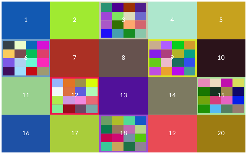

Partition is like Tiler, but you specify the width and height of the tiles, rather than how many rows and columns of tiles you want.

You can obtain the centerpoints of all the tiles in one go with:

first.(collect(tiles))

or obtain ranges with:

tiles[1:2:end]

Tables

The Table iterator can be used to define tables: rectangular grids with a specific number of rows and columns.

Unlike a Tiler, the Table iterator lets you have columns with different widths, and rows with different heights.

Tables don't store data, of course, but are designed to help you draw tabular data.

To create a simple table with 3 rows and 4 columns, using the default width and height (100):

julia> t = Table(3, 4);

When you use this as an iterator, you can get the coordinates of the center of each cell, and its number:

julia> for i in t
           println("row: $(t.currentrow), column: $(t.currentcol), center: $(i[1])")
       end
row: 1, column: 1, center: Luxor.Point(-150.0, -100.0)
row: 1, column: 2, center: Luxor.Point(-50.0, -100.0)
row: 1, column: 3, center: Luxor.Point(50.0, -100.0)
row: 1, column: 4, center: Luxor.Point(150.0, -100.0)
row: 2, column: 1, center: Luxor.Point(-150.0, 0.0)
row: 2, column: 2, center: Luxor.Point(-50.0, 0.0)
row: 2, column: 3, center: Luxor.Point(50.0, 0.0)
row: 2, column: 4, center: Luxor.Point(150.0, 0.0)
row: 3, column: 1, center: Luxor.Point(-150.0, 100.0)
row: 3, column: 2, center: Luxor.Point(-50.0, 100.0)
row: 3, column: 3, center: Luxor.Point(50.0, 100.0)
row: 3, column: 4, center: Luxor.Point(150.0, 100.0)

You can also access row and column information:

julia> for r in 1:size(t)[1]
           for c in 1:size(t)[2]
               @show t[r, c]
           end
       end
t[r, c] = Luxor.Point(-150.0, -100.0)
t[r, c] = Luxor.Point(-50.0, -100.0)
t[r, c] = Luxor.Point(50.0, -100.0)
t[r, c] = Luxor.Point(150.0, -100.0)
t[r, c] = Luxor.Point(-150.0, 0.0)
t[r, c] = Luxor.Point(-50.0, 0.0)
t[r, c] = Luxor.Point(50.0, 0.0)
t[r, c] = Luxor.Point(150.0, 0.0)
t[r, c] = Luxor.Point(-150.0, 100.0)
t[r, c] = Luxor.Point(-50.0, 100.0)
t[r, c] = Luxor.Point(50.0, 100.0)
t[r, c] = Luxor.Point(150.0, 100.0)

The next example creates a table with 10 rows and 10 columns, where each cell is 50 units wide and 35 high.

sethue("black")

t = Table(10, 10, 50, 35) # 10 rows, 10 columns, 50 wide, 35 high

hundred = 1:100

for n in 1:length(t)
   text(string(hundred[n]), t[n], halign=:center, valign=:middle)
end

setopacity(0.5)
sethue("thistle")
# row 3, every column
markcells(t, getcells(t, 3, :), func = (args...) -> (
        circle(args[1], args[2]/2, :fill)
    ), action=:stroke)

You can access rows or columns in the usual Julian way. See Selecting and highlighting cells for details about how to select and mark cells.

Notice that the table is drawn row by row, whereas 2D Julia arrays are usually accessed column by column.

Varying row heights and column widths

To specify varying row heights and column widths, supply arrays or ranges to the Table constructor. The next example has logarithmically increasing row heights, and four columns of width 130 points:

t = Table(10 .^ range(0.7, length=25, stop=1.5), fill(130, 4))

for (pt, n) in t
    setgray(rescale(n, 1, length(t), 0, 1))
    box(pt, t.colwidths[t.currentcol], t.rowheights[t.currentrow], :fill)
    sethue("white")
    fontsize(t.rowheights[t.currentrow])
    text(string(n), pt, halign=:center, valign=:middle)
end

To fill table cells, it's useful to be able to access the table's row and column specifications (using the colwidths and rowheights fields), and iteration can also provide information about the current row and column being processed (currentrow and currentcol).

To ensure that graphic elements don't stray outside the cell walls, you can use a clipping region.

Drawing arrays and dataframes

With a little bit of extra work you can write code that draws objects like arrays and dataframes combining text with graphic features. For example, this code draws arrays visually and numerically.

function drawbar(t::Table, data, row, column, minvalue, maxvalue, barheight)
    setline(1.5)
    cellwidth = t.colwidths[column] - 10
    leftmargin = t[row, column] - (cellwidth/2, 0)
    sethue("gray70")
    box(leftmargin - (0, barheight/2), leftmargin + (cellwidth, barheight/2), :fill)
    boxwidth = rescale(data[row, column], minvalue, maxvalue, 0, cellwidth)
    sethue("red")
    box(leftmargin - (0, barheight/2), leftmargin + (boxwidth, barheight/2), :fill)
    sethue("black")
    line(leftmargin + (boxwidth, -barheight/2),
         leftmargin + (boxwidth, +barheight/2),
         :stroke)
    text(string(round(data[row, column], digits=3)), t[row, column] - (cellwidth/2, 10),
         halign=:left)
end

A = rand(6, 6)
l, h = extrema(A)
rt, ct = size(A)
t = Table(size(A), (80, 30))
fontface("Georgia")
fontsize(12)
for r in 1:rt
    for c in 1:ct
        drawbar(t, A, r, c, l, h, 10)
    end
end

Selecting and highlighting cells

With getcells() and markcells() you can select and apply graphics to cells of Tables and Tilers.

getcells() has two ways to select cells: either by their single index value, or by specifying rows and columns. Remember, unlike with typical Julia arrays, in a 2 row by 4 column table, the cell at row 1, column 4 will have the index number 4, not 7:

 ┌───┬───┬───┬───┐
 │ 1 │ 2 │ 3 │ 4 │
 ├───┼───┼───┼───┤
 │ 5 │ 6 │ 7 │ 8 │
 └───┴───┴───┴───┘

The function returns an array of cells in Tuples, each Tuple holding the coordinate of the cell center and its index number.

The markcells() function takes a Table or Tiler, and the selected cells made by getcells(), and, by default, draws a box around each one. You can instead choose the :fill action, or supply a four-argument function that adds graphics relevant to the cell's position, width, height, and number.

@drawsvg begin
background("grey10")
fontsize(10)

t = Tiler(600, 300, 6, 6)

sethue("cyan")
# mark even cells
markcells(t, getcells(t, 2:2:36))

sethue("orange")
setopacity(0.5)
# fill odd cells orange
markcells(t, getcells(t, 1:2:35), action=:fill)

sethue("blue")
setopacity(0.5)
# fill cells in rows 2:5, columns 3:4 blue
markcells(t, getcells(t, 2:5, 3:4), action=:fill)
setopacity(1)

# draw circles and index numbers for primes
primes = filter(n -> all(i -> n % i != 0, 2:floor(Int, sqrt(n))), 2:36)
markcells(t, getcells(t, primes), func=(pt, w, h, n) -> begin
    sethue("purple")
    circle(pt, h / 2, :fill)
    sethue("white")
    text(string(n), pt, halign=:center, valign=:middle)
end)
end 600 300

Grids

You might also find a use for a grid. Luxor provides a simple grid utility. Grids are lazy: they'll supply the next point on the grid when you ask for it.

Define a rectangular grid with GridRect. Get the next grid point from a grid with nextgridpoint(grid).

grid = GridRect(O, 40, 80, (10 - 1) * 40)
for i in 1:20
    randomhue()
    p = nextgridpoint(grid)
    squircle(p, 20, 20, :fill)
    sethue("white")
    text(string(i), p, halign=:center)
end

Hexagonal grids

Use the hexagon constructors HexagonOffsetOddR, HexagonOffsetEvenR, HexagonAxial, and HexagonCubic to define a hexagonal tile on a grid, using hexagon index values to specify their location.

You can use hexcenter() to find the Cartesian coordinates of the center of a hexagonal tile on the grid, and hextile() to return the Cartesian coordinates of the vertices of the tile.

For example, this code draws a hexagon with the hexagonal indices 0 0 on a grid centred at the origin with grid spacing of 100 units:

sethue("purple")
poly(hextile(HexagonOffsetOddR(0, 0, 100)), :fill)

By default the hexagonal grid indices 0 0 are located at the drawing's origin (Point(0, 0)). You can change this, and also specify the width and height of the hexagonal grid.

By using different index values you can draw hexagons at other locations on the hexagonal grid.

sethue("purple")
poly(hextile(HexagonOffsetOddR(-1, -1, 40)), :fill)
sethue("orange")
poly(hextile(HexagonOffsetOddR(-1, 1, 40)), :fill)
sethue("green")
poly(hextile(HexagonOffsetOddR(1, 1, 40)), :fill)
sethue("blue")
poly(hextile(HexagonOffsetOddR(1, -1, 40)), :fill)

Hexagonal grid indexing

Whereas rectangular grids can be indexed using x ("column") and y ("row") integers, hexagonal grids can be indexed in various ways. For example, odd-numbered "rows" can be shifted to the right:

fontsize(16)
for q in -2:2 # vertical
    for r in -2:2 # horizontal
        pgon = hextile(HexagonOffsetOddR(q, r, 40))
        sethue(HSB(rand(1:360), 0.6, 0.7))
        poly(pgon, :fill)
        sethue("white")
        text("$q", hexcenter(HexagonOffsetOddR(q, r, 40)),
            halign=:left, valign=:top)
        text("$r", hexcenter(HexagonOffsetOddR(q, r, 40)),
            halign=:right, valign=:bottom)
    end
end

Alternatively, even-numbered "rows" can be shifted to the right:

fontsize(16)
for q in -2:2 # vertical
    for r in -2:2 # horizontal
        pgon = hextile(HexagonOffsetEvenR(q, r, 40))
        sethue(HSB(rand(1:360), 0.6, 0.7))
        poly(pgon, :fill)
        sethue("white")
        text("$q", hexcenter(HexagonOffsetEvenR(q, r, 40)),
            halign=:left, valign=:top)
        text("$r", hexcenter(HexagonOffsetEvenR(q, r, 40)),
            halign=:right, valign=:bottom)
    end
end

The cubic hexagon constructor accepts three coordinates:

for q in -2:2
    for r in -2:2
        pgon = hextile(HexagonCubic(q, r, -q - r, 25))
        sethue(HSB(rand(1:360), 0.6, 0.7))
        poly(pgon, :fill)
    end
end

The axial constructor accepts two:

for q in -2:2
    for r in -2:2
        pgon = hextile(HexagonAxial(q, r, 25))
        sethue(HSB(rand(1:360), 0.6, 0.7))
        poly(pgon, :fill)
    end
end

Hexagonal rings

The hexring() function finds the nth ring of adjacent hexagons surrounding a hexagon.

The first ring consists of six hexagons. Ring n consists of 6n hexagons.

hexa = HexagonOffsetOddR(0, 0, 10)
for i in 1:15
    ring = hexring(i, hexa)
    sethue(HSB(rescale(i, 1, 15, 0, 360), 0.8, 0.8))
    for (n, h) in enumerate(ring)
        poly(hextile(h), :fillpreserve)
    end
end

Neighbouring hexagons

To find the six hexagons that surround a hexagon, use hexneighbors().

for i in 1:10
    sethue(HSB(rand(0:360), 0.8, 0.8))
    hex1 = HexagonOffsetOddR(rand(-7:7), rand(-7:7), 15)
    for neighbor in hexneighbors(hex1)
        poly(hextile(neighbor), :fill)
        circle(hexcenter(neighbor), 25, :stroke)
    end
end

Spiralling hexagons

The hexspiral() function generates a spiral of hexagons around a central hexagon to form n rings of hexagons.

using Luxor, Colors
background("black")
hexagon = HexagonOffsetEvenR(0, 0, 16)
setline(0.75)
for (n, h) in enumerate(hexspiral(hexagon, 10))
    sethue(HSB(mod1(5n, 360), 0.8, 0.8))
    poly(hextile(h), :fillpreserve)
    sethue("black")
    text(string(n), hexcenter(h), halign=:center)
    strokepath()
end