Simple graphics
In Luxor, there are different ways of working with graphical items:
Draw them immediately. Create lines and curves to build a path on the drawing. When you paint the path, the graphics are ‘fixed’, and you move on to the next.
Construct arrays of points - polygons - which you can draw at some later point. Watch out for a
vertices=trueoption, which returns coordinate data rather than adding shapes to the current path.You can combine these two approaches: create a path from lines and curves (and jumps), then store the path, ready for drawing later on.
Line width
The default line width in Luxor is 2 points. (Typically 1 point is 0.352777mm, 1/72.0inch.) Set the line width with setline. Find the current line width with getline. By default, line widths don't vary depending on the current drawing scale, but you can ask for them to be scaled - see Scaling-of-line-thickness.
Rectangles and boxes
Simple rectangle and box shapes can be made in different ways.
rulers()
sethue("grey40")
rect(Point(0, 0), 100, 100, action = :stroke)
sethue("blue")
box(Point(0, 0), 100, 100, action=:stroke)
rect rectangles are positioned by a corner, a box made with box can be defined either by its center and dimensions, or by two opposite corners.
;fill-opacity:1;stroke:none;"/>
<path style="fill:none;stroke-width:2;stroke-linecap:butt;stroke-linejoin:miter;stroke:rgb(0%25,0%25,0%25);stroke-opacity:1;stroke-miterlimit:10;" d="M 30 195 L 30 55 L 170 55 L 170 195 Z M 30 195 "/>
<g style="fill:rgb(0%25,0%25,0%25);fill-opacity:1;">
<use xlink:href="%23glyph-8864910-1" x="67.345" y="215"/>
<use xlink:href="%23glyph-8864910-2" x="75.206" y="215"/>
<use xlink:href="%23glyph-8864910-3" x="83.158" y="215"/>
<use xlink:href="%23glyph-8864910-4" x="90.186" y="215"/>
<use xlink:href="%23glyph-8864910-5" x="93.938" y="215"/>
<use xlink:href="%23glyph-8864910-6" x="101.806" y="215"/>
<use xlink:href="%23glyph-8864910-7" x="109.926" y="215"/>
<use xlink:href="%23glyph-8864910-8" x="113.118" y="215"/>
<use xlink:href="%23glyph-8864910-5" x="116.667" y="215"/>
<use xlink:href="%23glyph-8864910-9" x="124.535" y="215"/>
</g>
<path style=" stroke:none;fill-rule:nonzero;fill:rgb(50.196078%25,0%25,50.196078%25);fill-opacity:1;" d="M 38 55 C 38 59.417969 34.417969 63 30 63 C 25.582031 63 22 59.417969 22 55 C 22 50.582031 25.582031 47 30 47 C 34.417969 47 38 50.582031 38 55 Z M 38 55 "/>
<path style=" stroke:none;fill-rule:nonzero;fill:rgb(50.196078%25,0%25,50.196078%25);fill-opacity:1;" d="M 178 195 C 178 199.417969 174.417969 203 170 203 C 165.582031 203 162 199.417969 162 195 C 162 190.582031 165.582031 187 170 187 C 174.417969 187 178 190.582031 178 195 Z M 178 195 "/>
<g style="fill:rgb(50.196078%25,0%25,50.196078%25);fill-opacity:1;">
<use xlink:href="%23glyph-8864910-5" x="22.006" y="32.613"/>
<use xlink:href="%23glyph-8864910-6" x="29.874" y="32.613"/>
</g>
<g style="fill:rgb(50.196078%25,0%25,50.196078%25);fill-opacity:1;">
<use xlink:href="%23glyph-8864910-5" x="162.006" y="225.157"/>
<use xlink:href="%23glyph-8864910-9" x="169.874" y="225.157"/>
</g>
<path style="fill:none;stroke-width:2;stroke-linecap:butt;stroke-linejoin:miter;stroke:rgb(0%25,0%25,0%25);stroke-opacity:1;stroke-miterlimit:10;" d="M 230 195 L 230 55 L 370 55 L 370 195 Z M 230 195 "/>
<g style="fill:rgb(0%25,0%25,0%25);fill-opacity:1;">
<use xlink:href="%23glyph-8864910-1" x="266.5995" y="215"/>
<use xlink:href="%23glyph-8864910-2" x="274.4605" y="215"/>
<use xlink:href="%23glyph-8864910-3" x="282.4125" y="215"/>
<use xlink:href="%23glyph-8864910-4" x="289.4405" y="215"/>
<use xlink:href="%23glyph-8864910-5" x="293.1925" y="215"/>
<use xlink:href="%23glyph-8864910-7" x="301.0605" y="215"/>
<use xlink:href="%23glyph-8864910-8" x="304.2525" y="215"/>
<use xlink:href="%23glyph-8864910-10" x="307.8015" y="215"/>
<use xlink:href="%23glyph-8864910-7" x="318.8335" y="215"/>
<use xlink:href="%23glyph-8864910-8" x="322.0255" y="215"/>
<use xlink:href="%23glyph-8864910-11" x="325.5745" y="215"/>
</g>
<path style=" stroke:none;fill-rule:nonzero;fill:rgb(50.196078%25,0%25,50.196078%25);fill-opacity:1;" d="M 308 125 C 308 129.417969 304.417969 133 300 133 C 295.582031 133 292 129.417969 292 125 C 292 120.582031 295.582031 117 300 117 C 304.417969 117 308 120.582031 308 125 Z M 308 125 "/>
<g style="fill:rgb(50.196078%25,0%25,50.196078%25);fill-opacity:1;">
<use xlink:href="%23glyph-8864910-5" x="296.066" y="152.231"/>
</g>
<path style="fill:none;stroke-width:1;stroke-linecap:butt;stroke-linejoin:miter;stroke:rgb(50.196078%25,0%25,50.196078%25);stroke-opacity:1;stroke-miterlimit:10;" d="M 230 40 L 360.761719 40 "/>
<path style=" stroke:none;fill-rule:nonzero;fill:rgb(50.196078%25,0%25,50.196078%25);fill-opacity:1;" d="M 360.761719 36.171875 L 370 40 L 360.761719 43.828125 "/>
<g style="fill:rgb(50.196078%25,0%25,50.196078%25);fill-opacity:1;">
<use xlink:href="%23glyph-8864910-10" x="300" y="30"/>
</g>
<path style="fill:none;stroke-width:1;stroke-linecap:butt;stroke-linejoin:miter;stroke:rgb(50.196078%25,0%25,50.196078%25);stroke-opacity:1;stroke-miterlimit:10;" d="M 215 55 L 215 185.761719 "/>
<path style=" stroke:none;fill-rule:nonzero;fill:rgb(50.196078%25,0%25,50.196078%25);fill-opacity:1;" d="M 218.828125 185.761719 L 215 195 L 211.171875 185.761719 "/>
<g style="fill:rgb(50.196078%25,0%25,50.196078%25);fill-opacity:1;">
<use xlink:href="%23glyph-8864910-11" x="205" y="125"/>
</g>
<path style="fill:none;stroke-width:2;stroke-linecap:butt;stroke-linejoin:miter;stroke:rgb(0%25,0%25,0%25);stroke-opacity:1;stroke-miterlimit:10;" d="M 430 195 L 430 55 L 570 55 L 570 195 Z M 430 195 "/>
<g style="fill:rgb(0%25,0%25,0%25);fill-opacity:1;">
<use xlink:href="%23glyph-8864910-12" x="463.3655" y="215"/>
<use xlink:href="%23glyph-8864910-13" x="468.4825" y="215"/>
<use xlink:href="%23glyph-8864910-14" x="475.8885" y="215"/>
<use xlink:href="%23glyph-8864910-15" x="482.5805" y="215"/>
<use xlink:href="%23glyph-8864910-4" x="487.6275" y="215"/>
<use xlink:href="%23glyph-8864910-5" x="491.3795" y="215"/>
<use xlink:href="%23glyph-8864910-15" x="499.2475" y="215"/>
<use xlink:href="%23glyph-8864910-7" x="504.2945" y="215"/>
<use xlink:href="%23glyph-8864910-8" x="507.4865" y="215"/>
<use xlink:href="%23glyph-8864910-10" x="511.0355" y="215"/>
<use xlink:href="%23glyph-8864910-7" x="522.0675" y="215"/>
<use xlink:href="%23glyph-8864910-8" x="525.2595" y="215"/>
<use xlink:href="%23glyph-8864910-11" x="528.8085" y="215"/>
</g>
<path style=" stroke:none;fill-rule:nonzero;fill:rgb(50.196078%25,0%25,50.196078%25);fill-opacity:1;" d="M 438 55 C 438 59.417969 434.417969 63 430 63 C 425.582031 63 422 59.417969 422 55 C 422 50.582031 425.582031 47 430 47 C 434.417969 47 438 50.582031 438 55 Z M 438 55 "/>
<g style="fill:rgb(50.196078%25,0%25,50.196078%25);fill-opacity:1;">
<use xlink:href="%23glyph-8864910-5" x="444.142136" y="78.529136"/>
<use xlink:href="%23glyph-8864910-15" x="452.010136" y="78.529136"/>
</g>
<path style="fill:none;stroke-width:1;stroke-linecap:butt;stroke-linejoin:miter;stroke:rgb(50.196078%25,0%25,50.196078%25);stroke-opacity:1;stroke-miterlimit:10;" d="M 430 40 L 560.761719 40 "/>
<path style=" stroke:none;fill-rule:nonzero;fill:rgb(50.196078%25,0%25,50.196078%25);fill-opacity:1;" d="M 560.761719 36.171875 L 570 40 L 560.761719 43.828125 "/>
<g style="fill:rgb(50.196078%25,0%25,50.196078%25);fill-opacity:1;">
<use xlink:href="%23glyph-8864910-10" x="500" y="30"/>
</g>
<path style="fill:none;stroke-width:1;stroke-linecap:butt;stroke-linejoin:miter;stroke:rgb(50.196078%25,0%25,50.196078%25);stroke-opacity:1;stroke-miterlimit:10;" d="M 415 55 L 415 185.761719 "/>
<path style=" stroke:none;fill-rule:nonzero;fill:rgb(50.196078%25,0%25,50.196078%25);fill-opacity:1;" d="M 418.828125 185.761719 L 415 195 L 411.171875 185.761719 "/>
<g style="fill:rgb(50.196078%25,0%25,50.196078%25);fill-opacity:1;">
<use xlink:href="%23glyph-8864910-11" x="405" y="125"/>
</g>
<path style="fill:none;stroke-width:2;stroke-linecap:butt;stroke-linejoin:miter;stroke:rgb(50.196078%25,0%25,50.196078%25);stroke-opacity:1;stroke-miterlimit:10;" d="M 721.632812 191.574219 L 689.183594 158.285156 L 643.367188 166.144531 L 665 125 L 643.367188 83.855469 L 689.183594 91.714844 L 721.632812 58.425781 L 728.316406 104.425781 L 770 125 L 728.316406 145.574219 Z M 721.632812 191.574219 "/>
<path style="fill:none;stroke-width:2;stroke-linecap:butt;stroke-linejoin:miter;stroke:rgb(0%25,0%25,0%25);stroke-opacity:1;stroke-miterlimit:10;" d="M 643.367188 191.574219 L 643.367188 58.425781 L 770 58.425781 L 770 191.574219 Z M 643.367188 191.574219 "/>
<g style="fill:rgb(0%25,0%25,0%25);fill-opacity:1;">
<use xlink:href="%23glyph-8864910-16" x="636.538" y="215"/>
<use xlink:href="%23glyph-8864910-2" x="645.617" y="215"/>
<use xlink:href="%23glyph-8864910-17" x="653.569" y="215"/>
<use xlink:href="%23glyph-8864910-18" x="661.388" y="215"/>
<use xlink:href="%23glyph-8864910-19" x="669.214" y="215"/>
<use xlink:href="%23glyph-8864910-20" x="677.075" y="215"/>
<use xlink:href="%23glyph-8864910-18" x="680.463" y="215"/>
<use xlink:href="%23glyph-8864910-21" x="688.289" y="215"/>
<use xlink:href="%23glyph-8864910-16" x="695.59" y="215"/>
<use xlink:href="%23glyph-8864910-2" x="704.669" y="215"/>
<use xlink:href="%23glyph-8864910-3" x="712.621" y="215"/>
<use xlink:href="%23glyph-8864910-4" x="719.649" y="215"/>
<use xlink:href="%23glyph-8864910-5" x="723.401" y="215"/>
<use xlink:href="%23glyph-8864910-2" x="731.269" y="215"/>
<use xlink:href="%23glyph-8864910-22" x="739.221" y="215"/>
<use xlink:href="%23glyph-8864910-23" x="742.553" y="215"/>
<use xlink:href="%23glyph-8864910-24" x="749.798" y="215"/>
<use xlink:href="%23glyph-8864910-24" x="753.102" y="215"/>
<use xlink:href="%23glyph-8864910-24" x="756.406" y="215"/>
<use xlink:href="%23glyph-8864910-25" x="759.71" y="215"/>
</g>
</g>
</svg>)
If you want the coordinates of the corners of a box, rather than draw one immediately, use:
box(centerpoint, width, height, vertices=true)or
box(corner1, corner2, vertices=true)box is also able to draw some of the other Luxor objects, such as BoundingBoxes and Table cells, and usually also returns the coordinates of the corners.
box(Point(0, 0), 100, 100)4-element Array{Point,1}:
Point(-50.0, 50.0)
Point(-50.0, -50.0)
Point(50.0, -50.0)
Point(50.0, 50.0)To draw a box/rectangle with rounded corners, supply one or four values for corner radii.
setline(6)
box(O, 200, 150, 10, action = :stroke) # 1 value for all corners
sethue("purple")
box(O, 260, 220, [0, 15, 40, 80], action = :stroke) # different for each
Or you could smooth the sharp corners of a box, like so:
setline(4)
polysmooth(box(O, 200, 150, vertices=true), 10, action = :stroke)
The squircle function makes nicer shapes.
Triangles, pentagons, and regular polygons
For regular polygons, pentagons, and so on, see the section on Polygons and paths. If you like drawing hexagons, you could also read Hexagonal grids.
Circles and ellipses
There are various ways to make circles, including by center and radius, or passing through two or three points:
sethue("black")
p1 = Point(0, -50)
p2 = Point(100, 0)
p3 = Point(0, 65)
map(p -> circle(p, 4, action = :fill), [p1, p2, p3])
sethue("orange")
circle(center3pts(p1, p2, p3)..., action = :stroke)

sethue("red")
p1 = Point(0, 30)
p2 = Point(20, -40)
p3 = Point(50, 5)
circle.((p1, p2, p3), 3, action = :stroke)
circle(p1, p2, p3, action = :stroke)
The center3pts function returns the center position and radius of a circle passing through three points:
sethue("black")
p1 = Point(0, -50)
p2 = Point(100, 0)
p3 = Point(0, 65)
map(p -> circle(p, 4, action = :fill), [p1, p2, p3])
sethue("orange")
circle(center3pts(p1, p2, p3)..., action = :stroke)
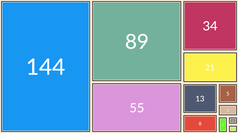
With ellipse you can place ellipses and circles by defining the center point and the width and height.
tiles = Tiler(500, 300, 5, 5)
width = 20
height = 25
for (pos, n) in tiles
    global width, height
    randomhue()
    ellipse(pos, width, height, action = :fill)
    sethue("black")
    label = string(round(width/height, digits=2))
    textcentered(label, pos.x, pos.y + 25)
    width += 2
end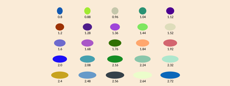
ellipse can also construct polygons that are approximations to ellipses. You supply two focal points and a length which is the sum of the distances of a point on the perimeter to the two focii.
fontface("Menlo")

f1 = Point(-100, 0)
f2 = Point(100, 0)

circle.([f1, f2], 3, action = :fill)

epoly = ellipse(f1, f2, 250, vertices=true)
poly(epoly, action = :stroke,  close=true)

pt = epoly[rand(1:end)]

poly([f1, pt, f2], action = :stroke)

label("f1", :W, f1, offset=10)
label("f2", :E, f2, offset=10)

label(string(round(distance(f1, pt), digits=1)), :SE, midpoint(f1, pt))
label(string(round(distance(pt, f2), digits=1)), :SW, midpoint(pt, f2))

label("ellipse(f1, f2, 250)", :S, Point(0, 75))
The advantage of this method is that there's a vertices=true option, allowing further scope for polygon manipulation.
f1 = Point(-100, 0)
f2 = Point(100, 0)
ellipsepoly = ellipse(f1, f2, 170, :none, vertices=true)
[ begin
    setgray(rescale(c, 150, 1, 0, 1))
    poly(offsetpoly(ellipsepoly, c), close=true, action = :fill);
    rotate(π/20)
  end
     for c in 150:-10:1 ]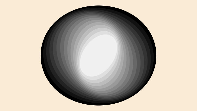
The ellipseinquad function constructs an ellipse that fits inside a four-sided quadrilateral.
pg = ngon(O, 250, 6, π/6, vertices=true)

top = vcat(O, pg[[3, 4, 5]])
left = vcat(O, pg[[1, 2, 3]])
right = vcat(O, pg[[5, 6, 1]])
sethue("red")
poly(top, action = :fill, close=true)

sethue("green")
poly(left, action = :fill, close=true)

sethue("blue")
poly(right, action = :fill, close=true)

sethue("orange")
ellipseinquad.((top, left, right), action = :fill)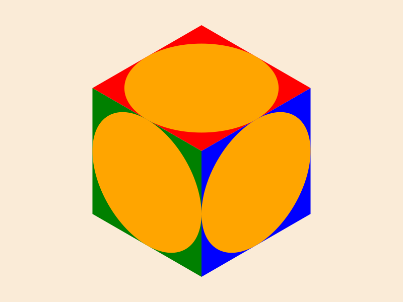
circlepath constructs a circular path from Bézier curves, which allows you to use circles as paths.
setline(4)
tiles = Tiler(600, 250, 1, 5)
for (pos, n) in tiles
    randomhue()
    circlepath(pos, tiles.tilewidth/2, action = :path)
    newsubpath()
    circlepath(pos, rand(5:tiles.tilewidth/2 - 1), action = :fill, reversepath=true)
end
Circles and tangents
Functions to find tangents to circles include:
pointcircletangentfinds a point on a circle that lies on line through another pointcirclecircleoutertangentsfinds the points that lie on outer tangents to two circlescirclecircleinnertangentsfinds the points that lie on inner tangents to two circlescircletangent2circlesmakes circles of a particular radius tangential to two circlescirclepointtangentmakes circles of a particular radius passing through a point and tangential to another circle
point = Point(-150, 0)
circlecenter = Point(150, 0)
circleradius = 80

circle.((point, circlecenter), 5, action = :fill)
circle(circlecenter, circleradius, action = :stroke)
pt1, pt2 = pointcircletangent(point, circlecenter, circleradius)
circle.((pt1, pt2), 5, action = :fill)

sethue("grey65")
rule(point, slope(point, pt1))
rule(point, slope(point, pt2))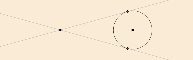
circle1center = Point(-150, 0)
circle1radius = 60
circle2center = Point(150, 0)
circle2radius = 80

circle.((circle1center, circle2center), 5, action = :fill)
circle(circle1center, circle1radius, action = :stroke)
circle(circle2center, circle2radius, action = :stroke)

p1, p2, p3, p4 = circlecircleoutertangents(
    circle1center, circle1radius,
    circle2center, circle2radius)

sethue("orange")
rule(p1, slope(p1, p2))
rule(p3, slope(p3, p4))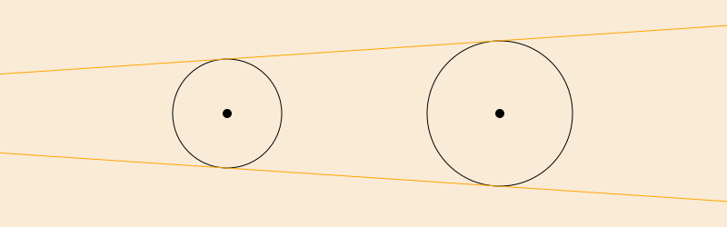
Finding the inner tangents requires a separate function.
circle1center = Point(-150, 0)
circle1radius = 60
circle2center = Point(150, 0)
circle2radius = 80

circle.((circle1center, circle2center), 5, action = :fill)
circle(circle1center, circle1radius, action = :stroke)
circle(circle2center, circle2radius, action = :stroke)

p1, p2, p3, p4 = circlecircleinnertangents(
    circle1center, circle1radius,
    circle2center, circle2radius)

label.(("p1", "p2", "p3", "p4"), :n, (p1, p2, p3, p4))
sethue("orange")
rule(p1, slope(p1, p2))
rule(p3, slope(p3, p4))

sethue("purple")
circle.((p1, p2, p3, p4), 3, action = :fill)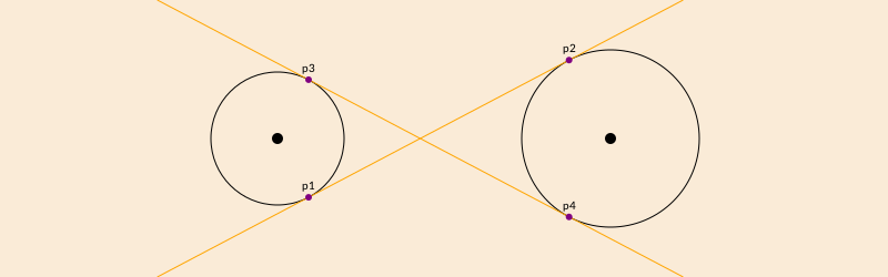
circletangent2circles takes the required radius and two existing circles:
circle1 = (Point(-100, 0), 90)
circle(circle1..., action = :stroke)
circle2 = (Point(100, 0), 90)
circle(circle2..., action = :stroke)

requiredradius = 25
ncandidates, p1, p2 = circletangent2circles(requiredradius, circle1..., circle2...)

if ncandidates==2
    sethue("orange")
    circle(p1, requiredradius, action = :fill)
    sethue("green")
    circle(p2, requiredradius, action = :fill)
    sethue("purple")
    circle(p1, requiredradius, action = :stroke)
    circle(p2, requiredradius, action = :stroke)
end

# the circles are 10 apart, so there should be just one circle
# that fits there

requiredradius = 10
ncandidates, p1, p2 = circletangent2circles(requiredradius, circle1..., circle2...)

if ncandidates==1
    sethue("blue")
    circle(p1, requiredradius, action = :fill)
    sethue("cyan")
    circle(p1, requiredradius, action = :stroke)
end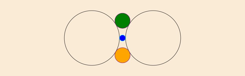
circlepointtangent looks for circles of a specified radius that pass through a point and are tangential to a circle. There are usually two candidates.
circle1 = (Point(-100, 0), 90)
circle(circle1..., action = :stroke)

requiredradius = 50
requiredpassthrough = O + (80, 0)
ncandidates, p1, p2 = circlepointtangent(requiredpassthrough, requiredradius, circle1...)

if ncandidates==2
    sethue("orange")
    circle(p1, requiredradius, action = :stroke)
    sethue("green")
    circle(p2, requiredradius, action = :stroke)
end

sethue("black")
circle(requiredpassthrough, 4, action = :fill)
These last two functions can return 0, 1, or 2 points (since there are often two solutions to a specific geometric layout).
circlering constructs n circles inside an outer circle and tangent to it. It returns both an array of 'circles' ((pt, radius) tuples), and details of the circle that fits inside them.
    background("grey10")
    sethue("rebeccapurple")
    setline(3)
    circle(Point(0, 0), 200, :stroke)
    cs, ic = circlering(Point(0, 0), 200, 10)
    for c in cs
        circle(first(c), last(c), :stroke)
    end
circle(first(ic), last(ic), :stroke);fill-opacity:1;stroke:none;"/>
<path style="fill:none;stroke-width:3;stroke-linecap:butt;stroke-linejoin:miter;stroke:rgb(40%25,20%25,60%25);stroke-opacity:1;stroke-miterlimit:10;" d="M 600 225 C 600 335.457031 510.457031 425 400 425 C 289.542969 425 200 335.457031 200 225 C 200 114.542969 289.542969 25 400 25 C 510.457031 25 600 114.542969 600 225 Z M 600 225 "/>
<path style="fill:none;stroke-width:3;stroke-linecap:butt;stroke-linejoin:miter;stroke:rgb(40%25,20%25,60%25);stroke-opacity:1;stroke-miterlimit:10;" d="M 570.820312 314.808594 C 570.820312 340.882812 549.683594 362.015625 523.609375 362.015625 C 497.535156 362.015625 476.398438 340.882812 476.398438 314.808594 C 476.398438 288.734375 497.535156 267.597656 523.609375 267.597656 C 549.683594 267.597656 570.820312 288.734375 570.820312 314.808594 Z M 570.820312 314.808594 "/>
<path style="fill:none;stroke-width:3;stroke-linecap:butt;stroke-linejoin:miter;stroke:rgb(40%25,20%25,60%25);stroke-opacity:1;stroke-miterlimit:10;" d="M 494.425781 370.3125 C 494.425781 396.386719 473.289062 417.523438 447.214844 417.523438 C 421.140625 417.523438 400.003906 396.386719 400.003906 370.3125 C 400.003906 344.238281 421.140625 323.101562 447.214844 323.101562 C 473.289062 323.101562 494.425781 344.238281 494.425781 370.3125 Z M 494.425781 370.3125 "/>
<path style="fill:none;stroke-width:3;stroke-linecap:butt;stroke-linejoin:miter;stroke:rgb(40%25,20%25,60%25);stroke-opacity:1;stroke-miterlimit:10;" d="M 399.996094 370.3125 C 399.996094 396.386719 378.859375 417.523438 352.785156 417.523438 C 326.710938 417.523438 305.574219 396.386719 305.574219 370.3125 C 305.574219 344.238281 326.710938 323.101562 352.785156 323.101562 C 378.859375 323.101562 399.996094 344.238281 399.996094 370.3125 Z M 399.996094 370.3125 "/>
<path style="fill:none;stroke-width:3;stroke-linecap:butt;stroke-linejoin:miter;stroke:rgb(40%25,20%25,60%25);stroke-opacity:1;stroke-miterlimit:10;" d="M 323.601562 314.808594 C 323.601562 340.882812 302.464844 362.015625 276.390625 362.015625 C 250.316406 362.015625 229.179688 340.882812 229.179688 314.808594 C 229.179688 288.734375 250.316406 267.597656 276.390625 267.597656 C 302.464844 267.597656 323.601562 288.734375 323.601562 314.808594 Z M 323.601562 314.808594 "/>
<path style="fill:none;stroke-width:3;stroke-linecap:butt;stroke-linejoin:miter;stroke:rgb(40%25,20%25,60%25);stroke-opacity:1;stroke-miterlimit:10;" d="M 294.417969 225 C 294.417969 251.074219 273.28125 272.210938 247.210938 272.210938 C 221.136719 272.210938 200 251.074219 200 225 C 200 198.925781 221.136719 177.789062 247.210938 177.789062 C 273.28125 177.789062 294.417969 198.925781 294.417969 225 Z M 294.417969 225 "/>
<path style="fill:none;stroke-width:3;stroke-linecap:butt;stroke-linejoin:miter;stroke:rgb(40%25,20%25,60%25);stroke-opacity:1;stroke-miterlimit:10;" d="M 323.601562 135.191406 C 323.601562 161.265625 302.464844 182.402344 276.390625 182.402344 C 250.316406 182.402344 229.179688 161.265625 229.179688 135.191406 C 229.179688 109.117188 250.316406 87.984375 276.390625 87.984375 C 302.464844 87.984375 323.601562 109.117188 323.601562 135.191406 Z M 323.601562 135.191406 "/>
<path style="fill:none;stroke-width:3;stroke-linecap:butt;stroke-linejoin:miter;stroke:rgb(40%25,20%25,60%25);stroke-opacity:1;stroke-miterlimit:10;" d="M 399.996094 79.6875 C 399.996094 105.761719 378.859375 126.898438 352.785156 126.898438 C 326.710938 126.898438 305.574219 105.761719 305.574219 79.6875 C 305.574219 53.613281 326.710938 32.476562 352.785156 32.476562 C 378.859375 32.476562 399.996094 53.613281 399.996094 79.6875 Z M 399.996094 79.6875 "/>
<path style="fill:none;stroke-width:3;stroke-linecap:butt;stroke-linejoin:miter;stroke:rgb(40%25,20%25,60%25);stroke-opacity:1;stroke-miterlimit:10;" d="M 494.425781 79.6875 C 494.425781 105.761719 473.289062 126.898438 447.214844 126.898438 C 421.140625 126.898438 400.003906 105.761719 400.003906 79.6875 C 400.003906 53.613281 421.140625 32.476562 447.214844 32.476562 C 473.289062 32.476562 494.425781 53.613281 494.425781 79.6875 Z M 494.425781 79.6875 "/>
<path style="fill:none;stroke-width:3;stroke-linecap:butt;stroke-linejoin:miter;stroke:rgb(40%25,20%25,60%25);stroke-opacity:1;stroke-miterlimit:10;" d="M 570.820312 135.191406 C 570.820312 161.265625 549.683594 182.402344 523.609375 182.402344 C 497.535156 182.402344 476.398438 161.265625 476.398438 135.191406 C 476.398438 109.117188 497.535156 87.984375 523.609375 87.984375 C 549.683594 87.984375 570.820312 109.117188 570.820312 135.191406 Z M 570.820312 135.191406 "/>
<path style="fill:none;stroke-width:3;stroke-linecap:butt;stroke-linejoin:miter;stroke:rgb(40%25,20%25,60%25);stroke-opacity:1;stroke-miterlimit:10;" d="M 600 225 C 600 251.074219 578.863281 272.210938 552.789062 272.210938 C 526.71875 272.210938 505.582031 251.074219 505.582031 225 C 505.582031 198.925781 526.71875 177.789062 552.789062 177.789062 C 578.863281 177.789062 600 198.925781 600 225 Z M 600 225 "/>
<path style="fill:none;stroke-width:3;stroke-linecap:butt;stroke-linejoin:miter;stroke:rgb(40%25,20%25,60%25);stroke-opacity:1;stroke-miterlimit:10;" d="M 505.582031 225 C 505.582031 283.3125 458.3125 330.582031 400 330.582031 C 341.6875 330.582031 294.417969 283.3125 294.417969 225 C 294.417969 166.6875 341.6875 119.417969 400 119.417969 C 458.3125 119.417969 505.582031 166.6875 505.582031 225 Z M 505.582031 225 "/>
</g>
</svg>)
Crescents
Use crescent to construct crescent shapes. There are two methods. The first method allows the two arcs to have the same radius. The second method allows the two arcs to share the same centers.
# method 1: same radius, different centers

sethue("purple")
crescent(Point(-200, 0), 200, Point(-150, 0), 200, action = :fill)

# method 2: same center, different radii

sethue("orange")
crescent(O, 100, 200, action = :fill)
Paths and positions
A path is a sequence of lines and curves. You can add lines and curves to the current path with various functions, then use closepath to join the last point to the first. Once you fill or stroke it, the path is emptied, and you start again.
A path can have subpaths, created withnewsubpath, which can form holes.
There is a 'current point' which you can set with move, and which is updated after functions like line, rline, rmove, text, newpath, closepath, arc, and curve. Use currentpoint and hascurrentpoint to find out about it.
You can store a path for later use with storepath and draw it with drawpath. See Stored paths.
For more about paths, see Polygons and paths and Paths versus polygons.
Lines
Use line and rline to draw straight lines. line(pt1, pt2, action) makes a path consisting of a line between two points. line(pt) adds a line to the current path going from the most recent current point to pt. rline(pt) adds a line relative to the current point.
You can use rule to draw a horizontal line through a point. Supply an angle for lines at an angle to the current x-axis.
y = 10
for x in 10 .^ range(0, length=100, stop=3)
    global y
    circle(Point(x, y), 2, action = :fill)
    rule(Point(x, y), -π/2, boundingbox=BoundingBox(centered=false))
    y += 2
end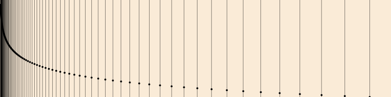
Use the boundingbox keyword argument to crop the ruled lines with a BoundingBox.
origin()
box(BoundingBox() * 0.9, action = :stroke)
for x in 10 .^ range(0, length=100, stop=3)
    rule(Point(x, 0), π/2,  boundingbox=BoundingBox() * 0.9)
    rule(Point(-x, 0), π/2, boundingbox=BoundingBox() * 0.9)
end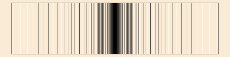
Arrows
You can draw lines, arcs, and curves with arrows at the end with arrow.
| type | function call |
|---|---|
| straight between two points | arrow(pt, pt) |
| curved: radius + two angles | arrow(pt, rad, θ1, θ2) |
| Bezier 4 points | arrow(pt1, pt2, pt3, pt4, action) |
| Bezier start finish + box | arrow(pt1, pt2, [ht1, ht2]) |
For straight arrows, supply the start and end points. For arrows as circular arcs, you provide center, radius, and start and finish angles. You can optionally provide dimensions for the arrowheadlength and arrowheadangle of the tip of the arrow (angle in radians between side and center). The default line weight is 1.0, equivalent to setline(1), but you can specify another.
arrow(Point(0, 0), Point(0, -65))
arrow(Point(0, 0), Point(100, -65), arrowheadlength=20, arrowheadangle=pi/4, linewidth=.3)
arrow(Point(0, 0), 100, π, π/2, arrowheadlength=25, arrowheadangle=pi/12, linewidth=1.25)![]()
If you provide four points, you can draw a Bézier curve with optional arrowheads at each end. Use the various options to control their presence and appearance.
pts = ngon(Point(0, 0), 100, 8, vertices=true)
sethue("mediumvioletred")
arrow(pts[2:5]..., :stroke, startarrow=false, finisharrow=true)
sethue("cyan4")
arrow(pts[3:6]..., startarrow=true, finisharrow=true)
sethue("midnightblue")
arrow(pts[[4, 2, 6, 8]]..., :stroke,
    startarrow=true,
    finisharrow=true,
    arrowheadangle = π/6,
    arrowheadlength = 35,
    linewidth  = 1.5)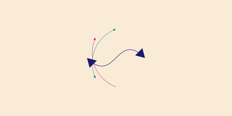
Decoration
The arrow functions allow you to specify decorations - graphics at one or more points somewhere along the shaft. For example, say you want to draw a number and a circle at the midpoint of an arrow's shaft, you can define a function that draws text t in a circle of radius r like this:
function marker(r, t)
    @layer begin
        sethue("purple")
        circle(Point(0, 0), r,  :fill)
        sethue("white")
        fontsize(30)
        text(string(t), halign=:center, valign=:middle)
    end
end
and then pass this to the decorate keyword argument of arrow. By default, the graphics origin when the function is called is placed at the midpoint (0.5) of the arrow's shaft.
pts = ngon(Point(0, 0), 100, 5, vertices=true)

sethue("mediumvioletred")

# using an anonymous function
arrow(pts[1:4]..., decorate = () -> marker(10, 3))

sethue("olivedrab")

# no arrow, just a graphic, at 0.75
arrow(pts[1:4]...,
    decorate = () ->
        ngon(Point(0, 0), 20, 4, 0, action = :fill),
    decoration = 0.75, :none) # default action is :stroke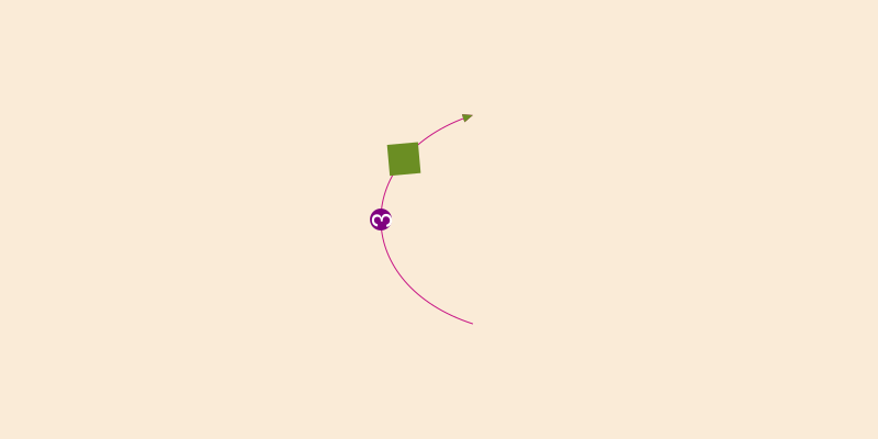
Use the decoration keyword to specify one or more locations other than the default 0.5.
The graphics environment provided by the decorate function is centered at each decoration point in turn, and rotated to the slope of the shaft at that point.
using Luxor

function fletcher()
    line(O, polar(30, deg2rad(220)), action = :stroke)
    line(O, polar(30, deg2rad(140)), action = :stroke)
end

@drawsvg begin
    background("antiquewhite")
        arrow(O, 150, 0, π + π/3,
            linewidth=5,
            arrowheadlength=50,
            decorate=fletcher,
            decoration=range(0., .1, length=3))
end 800 350;fill-opacity:1;stroke:none;"/>
<path style="fill:none;stroke-width:5;stroke-linecap:butt;stroke-linejoin:miter;stroke:rgb(0%25,0%25,0%25);stroke-opacity:1;stroke-miterlimit:10;" d="M 550 175 C 550 224.484375 525.59375 270.785156 484.769531 298.75 C 443.945312 326.714844 391.953125 332.746094 345.8125 314.871094 C 299.667969 296.992188 265.3125 257.507812 253.984375 209.339844 C 242.65625 161.167969 255.8125 110.507812 289.152344 73.941406 "/>
<path style=" stroke:none;fill-rule:nonzero;fill:rgb(0%25,0%25,0%25);fill-opacity:1;" d="M 277.015625 59.148438 L 325 45.097656 L 301.007812 88.960938 "/>
<path style="fill:none;stroke-width:5;stroke-linecap:butt;stroke-linejoin:miter;stroke:rgb(0%25,0%25,0%25);stroke-opacity:1;stroke-miterlimit:10;" d="M 550 175 L 569.285156 152.019531 "/>
<path style="fill:none;stroke-width:5;stroke-linecap:butt;stroke-linejoin:miter;stroke:rgb(0%25,0%25,0%25);stroke-opacity:1;stroke-miterlimit:10;" d="M 550 175 L 530.714844 152.019531 "/>
<path style="fill:none;stroke-width:5;stroke-linecap:butt;stroke-linejoin:miter;stroke:rgb(0%25,0%25,0%25);stroke-opacity:1;stroke-miterlimit:10;" d="M 547.183594 203.925781 L 570.539062 185.09375 "/>
<path style="fill:none;stroke-width:5;stroke-linecap:butt;stroke-linejoin:miter;stroke:rgb(0%25,0%25,0%25);stroke-opacity:1;stroke-miterlimit:10;" d="M 547.183594 203.925781 L 532.695312 177.65625 "/>
<path style="fill:none;stroke-width:5;stroke-linecap:butt;stroke-linejoin:miter;stroke:rgb(0%25,0%25,0%25);stroke-opacity:1;stroke-miterlimit:10;" d="M 538.84375 231.761719 L 565.390625 217.785156 "/>
<path style="fill:none;stroke-width:5;stroke-linecap:butt;stroke-linejoin:miter;stroke:rgb(0%25,0%25,0%25);stroke-opacity:1;stroke-miterlimit:10;" d="M 538.84375 231.761719 L 529.691406 203.191406 "/>
</g>
</svg>)
Custom arrowheads
To make custom arrowheads, you can define a three-argument function that draws them to your own design. This function takes the arguments:
the point at the end of the arrow's shaft
the point where the tip of the arrowhead would be
the angle of the shaft at the end
You can then use any code to draw the arrow. Pass this function to the arrow function's arrowheadfunction keyword.
function redbluearrow(shaftendpoint, endpoint, shaftangle)
    @layer begin
        sethue("red")
        sidept1 = shaftendpoint  + polar(10, shaftangle + π/2 )
        sidept2 = shaftendpoint  - polar(10, shaftangle + π/2)
        poly([sidept1, endpoint, sidept2], action=:fill)
        sethue("blue")
        poly([sidept1, endpoint, sidept2], action=:stroke, close=false)
    end
end

@drawsvg begin
    background("antiquewhite")
    arrow(O, O + (120, 120),
        linewidth=4,
        arrowheadlength=40,
        arrowheadangle=π/7,
        arrowheadfunction = redbluearrow)

    arrow(O, 100, 3π/2, π,
        linewidth=4,
        arrowheadlength=20,
        clockwise=false,arrowheadfunction=redbluearrow)
end 800 250;fill-opacity:1;stroke:none;"/>
<path style="fill:none;stroke-width:4;stroke-linecap:butt;stroke-linejoin:miter;stroke:rgb(0%25,0%25,0%25);stroke-opacity:1;stroke-miterlimit:10;" d="M 400 125 L 494.515625 219.515625 "/>
<path style="fill-rule:nonzero;fill:rgb(100%25,0%25,0%25);fill-opacity:1;stroke-width:4;stroke-linecap:butt;stroke-linejoin:miter;stroke:rgb(0%25,0%25,100%25);stroke-opacity:1;stroke-miterlimit:10;" d="M 487.445312 226.585938 L 520 245 L 501.585938 212.445312 "/>
<path style="fill:none;stroke-width:4;stroke-linecap:butt;stroke-linejoin:miter;stroke:rgb(0%25,0%25,0%25);stroke-opacity:1;stroke-miterlimit:10;" d="M 400 25 C 351.855469 25 310.546875 59.304688 301.703125 106.628906 "/>
<path style="fill-rule:nonzero;fill:rgb(100%25,0%25,0%25);fill-opacity:1;stroke-width:4;stroke-linecap:butt;stroke-linejoin:miter;stroke:rgb(0%25,0%25,100%25);stroke-opacity:1;stroke-miterlimit:10;" d="M 291.746094 105.703125 L 300 125 L 311.660156 107.550781 "/>
</g>
</svg>)
Arcs and curves
There are a few standard arc-drawing commands, such as curve, arc, carc, and arc2r. Because these are often used when building complex paths, they usually add arc sections to the current path. To construct a sequence of lines and arcs, use the :path action, followed by a final :stroke or similar.
curve constructs Bézier curves from control points:
setline(.5)
pt1 = Point(0, -125)
pt2 = Point(200, 125)
pt3 = Point(200, -125)

label.(string.(["O", "control point 1", "control point 2", "control point 3"]),
    :e,
    [O, pt1, pt2, pt3])

sethue("red")
map(p -> circle(p, 4, action=:fill), [O, pt1, pt2, pt3])

line(Point(0, 0), pt1, action=:stroke)
line(pt2, pt3, action = :stroke)

sethue("black")
setline(3)

# start a path
move(Point(0, 0))
curve(pt1, pt2, pt3) #  add to current path
strokepath()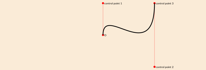
arc2r draws a circular arc centered at a point that passes through two other points:
tiles = Tiler(700, 200, 1, 6)
for (pos, n) in tiles
    c1, pt2, pt3 = ngon(pos, rand(10:50), 3, rand(0:pi/12:2pi), vertices=true)
    sethue("black")
    map(pt -> circle(pt, 4, action = :fill), [c1, pt3])
    sethue("red")
    circle(pt2, 4, action = :fill)
    randomhue()
    arc2r(c1, pt2, pt3, action = :stroke)
end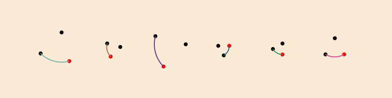
arc2sagitta and carc2sagitta make circular arcs based on two points and the sagitta.
pt1 = Point(-100, 0)
pt2 = Point(100, 0)
for n in reverse(range(1, length=7, stop=120))
    sethue("red")
    rule(Point(0, -n))
    sethue(LCHab(70, 80, rescale(n, 120, 1, 0, 359)))
    pt, r = arc2sagitta(pt1, pt2, n, action = :fillpreserve)
    sethue("black")
    strokepath()
    text(string(round(n)), O + (120, -n))
end
circle.((pt1, pt2), 5, action = :fill)
More curved shapes: sectors, spirals, and squircles
A sector (technically an "annular sector") has an inner and outer radius, as well as start and end angles.
sethue("tomato")
sector(50, 90, π/2, 0, action=:fill)
sethue("olive")
sector(Point(O.x + 200, O.y), 50, 90, 0, π/2, action=:fill)
You can also supply a value for a corner radius. The same sector is drawn but with rounded corners.
sethue("tomato")
sector(50, 90, π/2, 0, 15, action = :fill)
sethue("olive")
sector(Point(O.x + 200, O.y), 50, 90, 0, π/2, 15, action = :fill)
A pie (or wedge) has start and end angles.
pie(0, 0, 100, π/2, π, action = :fill)
To construct spirals, use the spiral function. These can be drawn directly, or used as polygons. The default is to draw Archimedean (non-logarithmic) spirals.
spiraldata = [
  (-2, "Lituus",      50),
  (-1, "Hyperbolic", 100),
  ( 1, "Archimedes",   1),
  ( 2, "Fermat",       5)]

grid = GridRect(O - (200, 0), 130, 50)

for aspiral in spiraldata
    @layer begin
        translate(nextgridpoint(grid))
        spiral(last(aspiral), first(aspiral), period=20π, action = :stroke)
        label(aspiral[2], :S, offset=100)
    end
end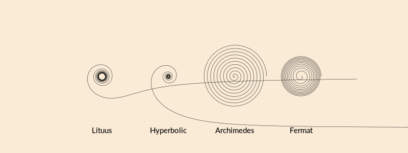
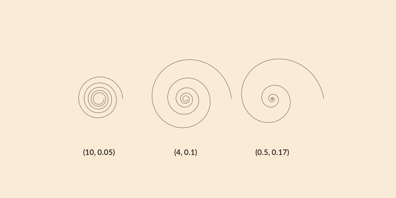
Use the log=true option to draw logarithmic (Bernoulli or Fibonacci) spirals.
spiraldata = [
    (10,  0.05),
    (4,   0.10),
    (0.5, 0.17)]

grid = GridRect(O - (200, 0), 175, 50)
for aspiral in spiraldata
    @layer begin
        translate(nextgridpoint(grid))
        spiral(first(aspiral), last(aspiral), log=true, period=10π, action = :stroke)
        label(string(aspiral), :S, offset=100)
    end
end
Modify the stepby and period parameters to taste, or collect the vertices for further processing.
A squircle is a cross between a square and a circle. You can adjust the squariness and circularity of it to taste by supplying a value for the root (keyword rt):
setline(2)
tiles = Tiler(600, 250, 1, 3)
for (pos, n) in tiles
    sethue("lavender")
    squircle(pos, 80, 80, rt=[0.3, 0.5, 0.7][n], action = :fillpreserve)
    sethue("grey20")
    strokepath()
    textcentered("rt = $([0.3, 0.5, 0.7][n])", pos)
end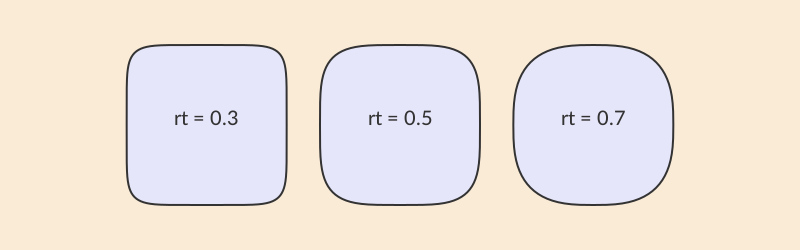
Stars and crosses
Use star to make a star. You can draw it immediately, or use the array of points it can create.
tiles = Tiler(400, 300, 4, 6, margin=5)
for (pos, n) in tiles
    randomhue()
    star(pos, tiles.tilewidth/3, rand(3:8), 0.5, 0, action = :fill)
end
The ratio determines the length of the inner radius compared with the outer.
tiles = Tiler(800, 250, 1, 6, margin=10)
for (pos, n) in tiles
    s = star(pos, tiles.tilewidth/2, 5, 1/n, 0, action = :stroke)
    l2 = distance(pos, s[1])
    l1 = distance(pos, s[2])
    text(string(round(l1/l2, digits=2)), pos, halign=:center)
end;fill-opacity:1;stroke:none;"/>
<path style="fill:none;stroke-width:2;stroke-linecap:butt;stroke-linejoin:miter;stroke:rgb(0%25,0%25,0%25);stroke-opacity:1;stroke-miterlimit:10;" d="M 95.085938 161.820312 L 54.914062 161.820312 L 22.414062 138.207031 L 10 100 L 22.414062 61.792969 L 54.914062 38.179688 L 95.085938 38.179688 L 127.585938 61.792969 L 140 100 L 127.585938 138.207031 Z M 95.085938 161.820312 "/>
<g style="fill:rgb(0%25,0%25,0%25);fill-opacity:1;">
<use xlink:href="%23glyph-3761100-1" x="68.02" y="100"/>
<use xlink:href="%23glyph-3761100-2" x="73.82" y="100"/>
<use xlink:href="%23glyph-3761100-3" x="76.18" y="100"/>
</g>
<path style="fill:none;stroke-width:2;stroke-linecap:butt;stroke-linejoin:miter;stroke:rgb(0%25,0%25,0%25);stroke-opacity:1;stroke-miterlimit:10;" d="M 225.085938 161.820312 L 194.957031 130.910156 L 152.414062 138.207031 L 172.5 100 L 152.414062 61.792969 L 194.957031 69.089844 L 225.085938 38.179688 L 231.292969 80.898438 L 270 100 L 231.292969 119.101562 Z M 225.085938 161.820312 "/>
<g style="fill:rgb(0%25,0%25,0%25);fill-opacity:1;">
<use xlink:href="%23glyph-3761100-3" x="198.02" y="100"/>
<use xlink:href="%23glyph-3761100-2" x="203.82" y="100"/>
<use xlink:href="%23glyph-3761100-4" x="206.18" y="100"/>
</g>
<path style="fill:none;stroke-width:2;stroke-linecap:butt;stroke-linejoin:miter;stroke:rgb(0%25,0%25,0%25);stroke-opacity:1;stroke-miterlimit:10;" d="M 355.085938 161.820312 L 328.304688 120.605469 L 282.414062 138.207031 L 313.332031 100 L 282.414062 61.792969 L 328.304688 79.394531 L 355.085938 38.179688 L 352.527344 87.265625 L 400 100 L 352.527344 112.734375 Z M 355.085938 161.820312 "/>
<g style="fill:rgb(0%25,0%25,0%25);fill-opacity:1;">
<use xlink:href="%23glyph-3761100-3" x="325.12" y="100"/>
<use xlink:href="%23glyph-3761100-2" x="330.92" y="100"/>
<use xlink:href="%23glyph-3761100-5" x="333.28" y="100"/>
<use xlink:href="%23glyph-3761100-5" x="339.08" y="100"/>
</g>
<path style="fill:none;stroke-width:2;stroke-linecap:butt;stroke-linejoin:miter;stroke:rgb(0%25,0%25,0%25);stroke-opacity:1;stroke-miterlimit:10;" d="M 485.085938 161.820312 L 459.976562 115.453125 L 412.414062 138.207031 L 448.75 100 L 412.414062 61.792969 L 459.976562 84.546875 L 485.085938 38.179688 L 478.148438 90.449219 L 530 100 L 478.148438 109.550781 Z M 485.085938 161.820312 "/>
<g style="fill:rgb(0%25,0%25,0%25);fill-opacity:1;">
<use xlink:href="%23glyph-3761100-3" x="455.12" y="100"/>
<use xlink:href="%23glyph-3761100-2" x="460.92" y="100"/>
<use xlink:href="%23glyph-3761100-6" x="463.28" y="100"/>
<use xlink:href="%23glyph-3761100-4" x="469.08" y="100"/>
</g>
<path style="fill:none;stroke-width:2;stroke-linecap:butt;stroke-linejoin:miter;stroke:rgb(0%25,0%25,0%25);stroke-opacity:1;stroke-miterlimit:10;" d="M 615.085938 161.820312 L 590.984375 112.363281 L 542.414062 138.207031 L 582 100 L 542.414062 61.792969 L 590.984375 87.636719 L 615.085938 38.179688 L 605.515625 92.359375 L 660 100 L 605.515625 107.640625 Z M 615.085938 161.820312 "/>
<g style="fill:rgb(0%25,0%25,0%25);fill-opacity:1;">
<use xlink:href="%23glyph-3761100-3" x="588.02" y="100"/>
<use xlink:href="%23glyph-3761100-2" x="593.82" y="100"/>
<use xlink:href="%23glyph-3761100-6" x="596.18" y="100"/>
</g>
<path style="fill:none;stroke-width:2;stroke-linecap:butt;stroke-linejoin:miter;stroke:rgb(0%25,0%25,0%25);stroke-opacity:1;stroke-miterlimit:10;" d="M 745.085938 161.820312 L 721.652344 110.304688 L 672.414062 138.207031 L 714.167969 100 L 672.414062 61.792969 L 721.652344 89.695312 L 745.085938 38.179688 L 733.765625 93.632812 L 790 100 L 733.765625 106.367188 Z M 745.085938 161.820312 "/>
<g style="fill:rgb(0%25,0%25,0%25);fill-opacity:1;">
<use xlink:href="%23glyph-3761100-3" x="715.12" y="100"/>
<use xlink:href="%23glyph-3761100-2" x="720.92" y="100"/>
<use xlink:href="%23glyph-3761100-1" x="723.28" y="100"/>
<use xlink:href="%23glyph-3761100-7" x="729.08" y="100"/>
</g>
</g>
</svg>)
Use polycross to draw a cross-shaped polygon.
tiles = Tiler(600, 600, 4, 4, margin=10)
for (pos, n) in tiles
    randomhue()
    polycross(pos, min(tiles.tileheight/3, tiles.tilewidth/3),
        n + 2, # number of points
        rescale(n, 1, length(tiles), 0.9, 0.1), # ratio
        0, # orientation
        action=:fill)
end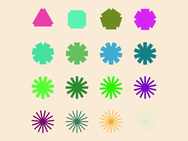
Stored paths
It's possible to store the current path in a Path object. For example, this code:
fontsize(160)
fontface("Bodoni-Poster")
textpath("†", O, halign=:center, valign=:middle)
dagger = storepath()
stores the instructions to build the current path (which describe the dagger symbol) in dagger.
The dagger is a Luxor Path type, and contains:
PathMove(Point(2.0, 90.5625)),
PathCurve(Point(4.08203125, 68.16015625), Point(11.28125, 45.28125), Point(24.8828125, 26.40234375)),
PathCurve(Point(17.51953125, 22.87890625), Point(2.0, 14.71875), Point(2.0, 5.12109375)),
PathCurve(Point(2.0, 2.5625), Point(3.12109375, 0.640625), Point(5.83984375, 0.640625)),
PathCurve(Point(12.8828125, 0.640625), Point(11.6015625, 14.2421875), Point(26.16015625, 14.2421875)),
PathCurve(Point(35.76171875, 14.2421875), Point(42.0, 7.83984375), Point(42.0, -1.59765625)),
PathCurve(Point(42.0, -10.3984375), Point(34.9609375, -17.4375), Point(26.16015625, -17.4375)),
PathCurve(Point(10.9609375, -17.4375), Point(13.04296875, -3.6796875), Point(6.48046875, -3.6796875)),
PathCurve(Point(3.6015625, -3.6796875), Point(1.83984375, -6.3984375), Point(1.83984375, -9.12109375)),
PathCurve(Point(1.83984375, -14.3984375), Point(12.2421875, -23.6796875), Point(15.44140625, -26.87890625)),
PathCurve(Point(18.640625, -30.078125), Point(19.76171875, -34.3984375), Point(19.76171875, -38.71875)),
PathCurve(Point(19.76171875, -49.7578125), Point(10.9609375, -56.640625), Point(0.40234375, -56.640625)),
PathCurve(Point(-11.1171875, -56.640625), Point(-19.91796875, -49.7578125), Point(-19.91796875, -38.71875)),
PathCurve(Point(-19.91796875, -34.3984375), Point(-18.80078125, -30.078125), Point(-15.59765625, -26.87890625)),
PathCurve(Point(-12.3984375, -23.6796875), Point(-2.0, -14.3984375), Point(-2.0, -9.12109375)),
PathCurve(Point(-2.0, -6.3984375), Point(-3.7578125, -3.6796875), Point(-6.640625, -3.6796875)),
PathCurve(Point(-13.19921875, -3.6796875), Point(-11.1171875, -17.4375), Point(-26.3203125, -17.4375)),
PathCurve(Point(-35.1171875, -17.4375), Point(-42.16015625, -10.3984375), Point(-42.16015625, -1.59765625)),
PathCurve(Point(-42.16015625, 7.83984375), Point(-35.91796875, 14.2421875), Point(-26.3203125, 14.2421875)),
PathCurve(Point(-11.7578125, 14.2421875), Point(-13.0390625, 0.640625), Point(-6.0, 0.640625)),
PathCurve(Point(-3.27734375, 0.640625), Point(-2.16015625, 2.5625), Point(-2.16015625, 5.12109375)),
PathCurve(Point(-2.16015625, 14.71875), Point(-17.6796875, 22.87890625), Point(-25.0390625, 26.40234375)),
PathCurve(Point(-11.4375, 45.28125), Point(-4.23828125, 68.16015625), Point(-2.16015625, 90.5625)),
PathClose(),
PathMove(Point(48.87890625, 56.640625))
You can draw this later:
for θ in range(0, step=2π/10, length=10)
    @layer begin
        rotate(θ)
        translate(150, 0)
        rotate(π/2)
        drawpath(dagger, action = :fill)
    end
end;fill-opacity:1;stroke:none;"/>
<path style=" stroke:none;fill-rule:nonzero;fill:rgb(0%25,0%25,0%25);fill-opacity:1;" d="M 359.4375 302 C 381.839844 304.082031 404.71875 311.28125 423.597656 324.882812 C 427.121094 317.519531 435.28125 302 444.878906 302 C 447.4375 302 449.359375 303.121094 449.359375 305.839844 C 449.359375 312.882812 435.757812 311.601562 435.757812 326.160156 C 435.757812 335.761719 442.160156 342 451.597656 342 C 460.398438 342 467.4375 334.960938 467.4375 326.160156 C 467.4375 310.960938 453.679688 313.042969 453.679688 306.480469 C 453.679688 303.601562 456.398438 301.839844 459.121094 301.839844 C 464.398438 301.839844 473.679688 312.242188 476.878906 315.441406 C 480.078125 318.640625 484.398438 319.761719 488.71875 319.761719 C 499.757812 319.761719 506.640625 310.960938 506.640625 300.402344 C 506.640625 288.882812 499.757812 280.082031 488.71875 280.082031 C 484.398438 280.082031 480.078125 281.199219 476.878906 284.402344 C 473.679688 287.601562 464.398438 298 459.121094 298 C 456.398438 298 453.679688 296.242188 453.679688 293.359375 C 453.679688 286.800781 467.4375 288.882812 467.4375 273.679688 C 467.4375 264.882812 460.398438 257.839844 451.597656 257.839844 C 442.160156 257.839844 435.757812 264.082031 435.757812 273.679688 C 435.757812 288.242188 449.359375 286.960938 449.359375 294 C 449.359375 296.722656 447.4375 297.839844 444.878906 297.839844 C 435.28125 297.839844 427.121094 282.320312 423.597656 274.960938 C 404.71875 288.5625 381.839844 295.761719 359.4375 297.839844 Z M 393.359375 348.878906 "/>
<path style=" stroke:none;fill-rule:nonzero;fill:rgb(0%25,0%25,0%25);fill-opacity:1;" d="M 346.910156 336.554688 C 363.808594 351.40625 378.089844 370.679688 385.367188 392.78125 C 392.546875 388.894531 408.269531 381.132812 416.035156 386.777344 C 418.105469 388.28125 419 390.316406 417.402344 392.515625 C 413.261719 398.214844 403.011719 389.183594 394.453125 400.960938 C 388.808594 408.726562 390.324219 417.539062 397.957031 423.085938 C 405.078125 428.257812 414.910156 426.703125 420.082031 419.582031 C 429.015625 407.285156 416.664062 400.882812 420.519531 395.574219 C 422.210938 393.246094 425.449219 393.417969 427.648438 395.015625 C 431.917969 398.121094 433.3125 411.992188 434.023438 416.460938 C 434.730469 420.929688 437.566406 424.375 441.0625 426.914062 C 449.992188 433.402344 460.734375 430.328125 466.9375 421.785156 C 473.710938 412.464844 473.316406 401.300781 464.382812 394.8125 C 460.890625 392.273438 456.738281 390.636719 452.265625 391.347656 C 447.796875 392.054688 434.175781 395.011719 429.90625 391.910156 C 427.703125 390.3125 426.539062 387.289062 428.234375 384.957031 C 432.085938 379.652344 441.996094 389.421875 450.929688 377.125 C 456.101562 370.007812 454.546875 360.171875 447.425781 355 C 439.792969 349.453125 430.941406 350.738281 425.300781 358.503906 C 416.742188 370.285156 428.5 377.242188 424.359375 382.9375 C 422.761719 385.140625 420.550781 384.914062 418.480469 383.410156 C 410.714844 377.769531 413.234375 360.417969 414.710938 352.390625 C 391.441406 352.300781 368.699219 344.675781 349.355469 333.1875 Z M 346.800781 394.417969 "/>
<path style=" stroke:none;fill-rule:nonzero;fill:rgb(0%25,0%25,0%25);fill-opacity:1;" d="M 316.464844 357.144531 C 321.40625 379.097656 321.628906 403.078125 314.527344 425.238281 C 322.621094 426.3125 339.902344 429.277344 342.867188 438.40625 C 343.660156 440.839844 343.1875 443.015625 340.601562 443.855469 C 333.902344 446.03125 330.917969 432.699219 317.070312 437.199219 C 307.941406 440.164062 303.984375 448.179688 306.902344 457.15625 C 309.621094 465.527344 318.492188 470.046875 326.859375 467.328125 C 341.316406 462.628906 335.085938 450.1875 341.328125 448.160156 C 344.0625 447.269531 346.578125 449.3125 347.421875 451.902344 C 349.050781 456.921875 342.027344 468.960938 339.972656 472.992188 C 337.917969 477.023438 338.1875 481.480469 339.523438 485.589844 C 342.933594 496.085938 353.429688 499.914062 363.472656 496.652344 C 374.429688 493.089844 380.671875 483.824219 377.261719 473.328125 C 375.925781 469.21875 373.527344 465.453125 369.492188 463.402344 C 365.460938 461.347656 352.703125 455.734375 351.074219 450.714844 C 350.230469 448.125 351.0625 444.996094 353.804688 444.105469 C 360.042969 442.078125 362.3125 455.808594 376.773438 451.109375 C 385.140625 448.390625 389.664062 439.519531 386.941406 431.148438 C 384.027344 422.175781 376.113281 418.015625 366.984375 420.980469 C 353.132812 425.480469 358.554688 438.019531 351.859375 440.195312 C 349.273438 441.035156 347.613281 439.554688 346.824219 437.121094 C 343.859375 427.992188 356.097656 415.4375 362.007812 409.8125 C 343.238281 396.058594 329.320312 376.523438 320.421875 355.859375 Z M 282.363281 403.894531 "/>
<path style=" stroke:none;fill-rule:nonzero;fill:rgb(0%25,0%25,0%25);fill-opacity:1;" d="M 279.730469 355.910156 C 270.828125 376.574219 256.910156 396.105469 238.140625 409.859375 C 244.054688 415.484375 256.292969 428.042969 253.328125 437.171875 C 252.539062 439.601562 250.878906 441.085938 248.292969 440.246094 C 241.59375 438.066406 247.015625 425.527344 233.167969 421.03125 C 224.039062 418.0625 216.125 422.222656 213.210938 431.199219 C 210.488281 439.570312 215.007812 448.4375 223.378906 451.160156 C 237.835938 455.855469 240.105469 442.128906 246.347656 444.15625 C 249.085938 445.046875 249.921875 448.175781 249.078125 450.765625 C 247.449219 455.785156 234.6875 461.394531 230.65625 463.449219 C 226.625 465.503906 224.222656 469.265625 222.886719 473.375 C 219.476562 483.875 225.71875 493.140625 235.761719 496.402344 C 246.71875 499.960938 257.214844 496.136719 260.625 485.636719 C 261.960938 481.527344 262.234375 477.074219 260.175781 473.042969 C 258.121094 469.011719 251.101562 456.96875 252.730469 451.953125 C 253.574219 449.363281 256.085938 447.320312 258.824219 448.210938 C 265.0625 450.238281 258.832031 462.679688 273.292969 467.375 C 281.65625 470.09375 290.53125 465.578125 293.25 457.207031 C 296.167969 448.230469 292.207031 440.210938 283.082031 437.246094 C 269.230469 432.746094 266.246094 446.078125 259.550781 443.902344 C 256.960938 443.0625 256.492188 440.890625 257.285156 438.457031 C 260.25 429.328125 277.53125 426.363281 285.621094 425.285156 C 278.519531 403.128906 278.742188 379.144531 283.6875 357.195312 Z M 224.664062 373.6875 "/>
<path style=" stroke:none;fill-rule:nonzero;fill:rgb(0%25,0%25,0%25);fill-opacity:1;" d="M 250.738281 333.320312 C 231.390625 344.800781 208.648438 352.425781 185.382812 352.519531 C 186.859375 360.546875 189.378906 377.898438 181.613281 383.539062 C 179.546875 385.042969 177.332031 385.265625 175.734375 383.066406 C 171.59375 377.367188 183.351562 370.410156 174.792969 358.632812 C 169.148438 350.863281 160.304688 349.582031 152.667969 355.128906 C 145.546875 360.300781 143.992188 370.132812 149.164062 377.253906 C 158.097656 389.550781 168.003906 379.777344 171.863281 385.085938 C 173.554688 387.417969 172.390625 390.441406 170.1875 392.039062 C 165.917969 395.140625 152.292969 392.183594 147.824219 391.472656 C 143.355469 390.765625 139.203125 392.398438 135.707031 394.9375 C 126.777344 401.425781 126.382812 412.59375 132.585938 421.136719 C 139.359375 430.453125 150.101562 433.527344 159.03125 427.039062 C 162.527344 424.5 165.363281 421.058594 166.070312 416.585938 C 166.777344 412.117188 168.175781 398.25 172.445312 395.148438 C 174.648438 393.546875 177.878906 393.371094 179.574219 395.703125 C 183.429688 401.007812 171.074219 407.410156 180.011719 419.710938 C 185.179688 426.828125 195.015625 428.386719 202.136719 423.214844 C 209.769531 417.667969 211.28125 408.855469 205.640625 401.089844 C 197.082031 389.308594 186.828125 398.339844 182.691406 392.644531 C 181.09375 390.441406 181.992188 388.410156 184.058594 386.90625 C 191.824219 381.265625 207.546875 389.023438 214.726562 392.90625 C 222.003906 370.804688 236.28125 351.53125 253.183594 336.683594 Z M 195.742188 315.332031 "/>
<path style=" stroke:none;fill-rule:nonzero;fill:rgb(0%25,0%25,0%25);fill-opacity:1;" d="M 240.5625 298 C 218.160156 295.917969 195.28125 288.71875 176.402344 275.117188 C 172.878906 282.480469 164.71875 298 155.121094 298 C 152.5625 298 150.640625 296.878906 150.640625 294.160156 C 150.640625 287.117188 164.242188 288.398438 164.242188 273.839844 C 164.242188 264.238281 157.839844 258 148.402344 258 C 139.601562 258 132.5625 265.039062 132.5625 273.839844 C 132.5625 289.039062 146.320312 286.957031 146.320312 293.519531 C 146.320312 296.398438 143.601562 298.160156 140.878906 298.160156 C 135.601562 298.160156 126.320312 287.757812 123.121094 284.558594 C 119.921875 281.359375 115.601562 280.238281 111.28125 280.238281 C 100.242188 280.238281 93.359375 289.039062 93.359375 299.597656 C 93.359375 311.117188 100.242188 319.917969 111.28125 319.917969 C 115.601562 319.917969 119.921875 318.800781 123.121094 315.597656 C 126.320312 312.398438 135.601562 302 140.878906 302 C 143.601562 302 146.320312 303.757812 146.320312 306.640625 C 146.320312 313.199219 132.5625 311.117188 132.5625 326.320312 C 132.5625 335.117188 139.601562 342.160156 148.402344 342.160156 C 157.839844 342.160156 164.242188 335.917969 164.242188 326.320312 C 164.242188 311.757812 150.640625 313.039062 150.640625 306 C 150.640625 303.277344 152.5625 302.160156 155.121094 302.160156 C 164.71875 302.160156 172.878906 317.679688 176.402344 325.039062 C 195.28125 311.4375 218.160156 304.238281 240.5625 302.160156 Z M 206.640625 251.121094 "/>
<path style=" stroke:none;fill-rule:nonzero;fill:rgb(0%25,0%25,0%25);fill-opacity:1;" d="M 253.089844 263.445312 C 236.191406 248.59375 221.910156 229.320312 214.632812 207.21875 C 207.453125 211.105469 191.730469 218.867188 183.964844 213.222656 C 181.894531 211.71875 181 209.683594 182.597656 207.484375 C 186.738281 201.785156 196.988281 210.816406 205.546875 199.039062 C 211.191406 191.273438 209.675781 182.460938 202.042969 176.914062 C 194.921875 171.742188 185.089844 173.296875 179.917969 180.417969 C 170.984375 192.714844 183.335938 199.117188 179.480469 204.425781 C 177.789062 206.753906 174.550781 206.582031 172.351562 204.984375 C 168.082031 201.878906 166.6875 188.007812 165.976562 183.539062 C 165.269531 179.070312 162.433594 175.625 158.9375 173.085938 C 150.007812 166.597656 139.265625 169.671875 133.0625 178.214844 C 126.289062 187.535156 126.683594 198.699219 135.617188 205.1875 C 139.109375 207.726562 143.261719 209.363281 147.734375 208.652344 C 152.203125 207.945312 165.824219 204.988281 170.09375 208.089844 C 172.296875 209.6875 173.460938 212.710938 171.765625 215.042969 C 167.914062 220.347656 158.003906 210.578125 149.070312 222.875 C 143.898438 229.992188 145.453125 239.828125 152.574219 245 C 160.207031 250.546875 169.058594 249.261719 174.699219 241.496094 C 183.257812 229.714844 171.5 222.757812 175.640625 217.0625 C 177.238281 214.859375 179.449219 215.085938 181.519531 216.589844 C 189.285156 222.230469 186.765625 239.582031 185.289062 247.609375 C 208.558594 247.699219 231.300781 255.324219 250.644531 266.8125 Z M 253.199219 205.582031 "/>
<path style=" stroke:none;fill-rule:nonzero;fill:rgb(0%25,0%25,0%25);fill-opacity:1;" d="M 283.535156 242.855469 C 278.59375 220.902344 278.371094 196.921875 285.472656 174.761719 C 277.378906 173.6875 260.097656 170.722656 257.132812 161.59375 C 256.339844 159.160156 256.8125 156.984375 259.398438 156.144531 C 266.097656 153.96875 269.082031 167.300781 282.929688 162.800781 C 292.058594 159.835938 296.015625 151.820312 293.097656 142.84375 C 290.378906 134.472656 281.507812 129.953125 273.140625 132.671875 C 258.683594 137.371094 264.914062 149.8125 258.671875 151.839844 C 255.9375 152.730469 253.421875 150.6875 252.578125 148.097656 C 250.949219 143.078125 257.972656 131.039062 260.027344 127.007812 C 262.082031 122.976562 261.8125 118.519531 260.476562 114.410156 C 257.066406 103.914062 246.570312 100.085938 236.527344 103.347656 C 225.570312 106.910156 219.328125 116.175781 222.738281 126.671875 C 224.074219 130.78125 226.472656 134.546875 230.507812 136.597656 C 234.539062 138.652344 247.296875 144.265625 248.925781 149.285156 C 249.769531 151.875 248.9375 155.003906 246.195312 155.894531 C 239.957031 157.921875 237.6875 144.191406 223.226562 148.890625 C 214.859375 151.609375 210.335938 160.480469 213.058594 168.851562 C 215.972656 177.824219 223.886719 181.984375 233.015625 179.019531 C 246.867188 174.519531 241.445312 161.980469 248.140625 159.804688 C 250.726562 158.964844 252.386719 160.445312 253.175781 162.878906 C 256.140625 172.007812 243.902344 184.5625 237.992188 190.1875 C 256.761719 203.941406 270.679688 223.476562 279.578125 244.140625 Z M 317.636719 196.105469 "/>
<path style=" stroke:none;fill-rule:nonzero;fill:rgb(0%25,0%25,0%25);fill-opacity:1;" d="M 320.269531 244.089844 C 329.171875 223.425781 343.089844 203.894531 361.859375 190.140625 C 355.945312 184.515625 343.707031 171.957031 346.671875 162.828125 C 347.460938 160.398438 349.121094 158.914062 351.707031 159.753906 C 358.40625 161.933594 352.984375 174.472656 366.832031 178.96875 C 375.960938 181.9375 383.875 177.777344 386.789062 168.800781 C 389.511719 160.429688 384.992188 151.5625 376.621094 148.839844 C 362.164062 144.144531 359.894531 157.871094 353.652344 155.84375 C 350.914062 154.953125 350.078125 151.824219 350.921875 149.234375 C 352.550781 144.214844 365.3125 138.605469 369.34375 136.550781 C 373.375 134.496094 375.777344 130.734375 377.113281 126.625 C 380.523438 116.125 374.28125 106.859375 364.238281 103.597656 C 353.28125 100.039062 342.785156 103.863281 339.375 114.363281 C 338.039062 118.472656 337.765625 122.925781 339.824219 126.957031 C 341.878906 130.988281 348.898438 143.03125 347.269531 148.046875 C 346.425781 150.636719 343.914062 152.679688 341.175781 151.789062 C 334.9375 149.761719 341.167969 137.320312 326.707031 132.625 C 318.34375 129.90625 309.46875 134.421875 306.75 142.792969 C 303.832031 151.769531 307.792969 159.789062 316.917969 162.753906 C 330.769531 167.253906 333.753906 153.921875 340.449219 156.097656 C 343.039062 156.9375 343.507812 159.109375 342.714844 161.542969 C 339.75 170.671875 322.46875 173.636719 314.378906 174.714844 C 321.480469 196.871094 321.257812 220.855469 316.3125 242.804688 Z M 375.335938 226.3125 "/>
<path style=" stroke:none;fill-rule:nonzero;fill:rgb(0%25,0%25,0%25);fill-opacity:1;" d="M 349.261719 266.679688 C 368.609375 255.199219 391.351562 247.574219 414.617188 247.480469 C 413.140625 239.453125 410.621094 222.101562 418.386719 216.460938 C 420.453125 214.957031 422.667969 214.734375 424.265625 216.933594 C 428.40625 222.632812 416.648438 229.589844 425.207031 241.367188 C 430.851562 249.136719 439.695312 250.417969 447.332031 244.871094 C 454.453125 239.699219 456.007812 229.867188 450.835938 222.746094 C 441.902344 210.449219 431.996094 220.222656 428.136719 214.914062 C 426.445312 212.582031 427.609375 209.558594 429.8125 207.960938 C 434.082031 204.859375 447.707031 207.816406 452.175781 208.527344 C 456.644531 209.234375 460.796875 207.601562 464.292969 205.0625 C 473.222656 198.574219 473.617188 187.40625 467.414062 178.863281 C 460.640625 169.546875 449.898438 166.472656 440.96875 172.960938 C 437.472656 175.5 434.636719 178.941406 433.929688 183.414062 C 433.222656 187.882812 431.824219 201.75 427.554688 204.851562 C 425.351562 206.453125 422.121094 206.628906 420.425781 204.296875 C 416.570312 198.992188 428.925781 192.589844 419.988281 180.289062 C 414.820312 173.171875 404.984375 171.613281 397.863281 176.785156 C 390.230469 182.332031 388.71875 191.144531 394.359375 198.910156 C 402.917969 210.691406 413.171875 201.660156 417.308594 207.355469 C 418.90625 209.558594 418.007812 211.589844 415.941406 213.09375 C 408.175781 218.734375 392.453125 210.976562 385.273438 207.09375 C 377.996094 229.195312 363.71875 248.46875 346.816406 263.316406 Z M 404.257812 284.667969 "/>
</g>
</svg>)
After you've stored the current path, it's still active. You might want to use newpath() before starting the next one. The drawpath() function will by default start a new path but there is an option to continue drawing the current one.
Other functions for working with stored paths include:
drawpathdraw all or part of a stored path using the current graphics statepathsampleresample the stored pathpathlengthfind the length of a stored pathBoundingBoxfind the bounding box of a stored path
Julia logos
A couple of functions, julialogo and juliacircles, provide you with instant access to the Julia logo and the three colored circles/dots:
cells = Table([300], [350, 350])

@layer begin
    translate(cells[1])
    translate(-165, -114)
    rulers()
    julialogo()
end

@layer begin
    translate(cells[2])
    translate(-165, -114)
    rulers()
    julialogo(action=:clip)
    for i in 1:500
        @layer begin
            translate(rand(0:400), rand(0:250))
            juliacircles(10)
        end
    end
    clipreset()
end![]()
There are various options for julialogo() to control coloring and positioning.
The four standard Julia colors are available as RGB tuples as Luxor.julia_blue, Luxor.julia_green, Luxor.julia_purple, Luxor.julia_red:
julia> Luxor.julia_red
(0.796, 0.235, 0.2)
Hypotrochoids
hypotrochoid makes hypotrochoids. The result is a polygon. You can either draw it directly, or pass it on for further polygon fun, as here, which uses offsetpoly to trace round it a few times.
origin()
background("grey15")
sethue("antiquewhite")
setline(1)
p = hypotrochoid(100, 25, 55, action = :stroke, stepby=0.01, vertices=true)
for i in 0:3:15
    poly(offsetpoly(p, i), action = :stroke, close=true)
end
There's a matching epitrochoid function.
Ticks
The tickline function lets you divide the space between two points by drawing ‘ticks’, short parallel lines positioned equidistant between the two points.
In its simplest form the function can used to draw basic number lines, complete with automatic text labels.
background("antiquewhite")

# major defaults to 1
tickline(Point(-350, -100), Point(350, -100))

# three major ticks inserted
tickline(Point(-350, 0), Point(350, 0),
    major=3,
    startnumber=0, finishnumber=100)

# four minor ticks inserted between each major
tickline(Point(-350, 100), Point(350, 100), major=3, minor=4);fill-opacity:1;stroke:none;"/>
<path style="fill:none;stroke-width:2;stroke-linecap:butt;stroke-linejoin:miter;stroke:rgb(0%25,0%25,0%25);stroke-opacity:1;stroke-miterlimit:10;" d="M 50 75 L 750 75 "/>
<path style="fill:none;stroke-width:2;stroke-linecap:butt;stroke-linejoin:miter;stroke:rgb(0%25,0%25,0%25);stroke-opacity:1;stroke-miterlimit:10;" d="M 50 75 L 50 95 "/>
<g style="fill:rgb(0%25,0%25,0%25);fill-opacity:1;">
<use xlink:href="%23glyph-5668350-1" x="43.02" y="108.255"/>
<use xlink:href="%23glyph-5668350-2" x="48.82" y="108.255"/>
<use xlink:href="%23glyph-5668350-1" x="51.18" y="108.255"/>
</g>
<path style="fill:none;stroke-width:2;stroke-linecap:butt;stroke-linejoin:miter;stroke:rgb(0%25,0%25,0%25);stroke-opacity:1;stroke-miterlimit:10;" d="M 400 75 L 400 95 "/>
<g style="fill:rgb(0%25,0%25,0%25);fill-opacity:1;">
<use xlink:href="%23glyph-5668350-1" x="393.02" y="108.255"/>
<use xlink:href="%23glyph-5668350-2" x="398.82" y="108.255"/>
<use xlink:href="%23glyph-5668350-3" x="401.18" y="108.255"/>
</g>
<path style="fill:none;stroke-width:2;stroke-linecap:butt;stroke-linejoin:miter;stroke:rgb(0%25,0%25,0%25);stroke-opacity:1;stroke-miterlimit:10;" d="M 750 75 L 750 95 "/>
<g style="fill:rgb(0%25,0%25,0%25);fill-opacity:1;">
<use xlink:href="%23glyph-5668350-4" x="743.02" y="108.255"/>
<use xlink:href="%23glyph-5668350-2" x="748.82" y="108.255"/>
<use xlink:href="%23glyph-5668350-1" x="751.18" y="108.255"/>
</g>
<path style="fill:none;stroke-width:2;stroke-linecap:butt;stroke-linejoin:miter;stroke:rgb(0%25,0%25,0%25);stroke-opacity:1;stroke-miterlimit:10;" d="M 50 175 L 750 175 "/>
<path style="fill:none;stroke-width:2;stroke-linecap:butt;stroke-linejoin:miter;stroke:rgb(0%25,0%25,0%25);stroke-opacity:1;stroke-miterlimit:10;" d="M 50 175 L 50 195 "/>
<g style="fill:rgb(0%25,0%25,0%25);fill-opacity:1;">
<use xlink:href="%23glyph-5668350-1" x="43.02" y="208.255"/>
<use xlink:href="%23glyph-5668350-2" x="48.82" y="208.255"/>
<use xlink:href="%23glyph-5668350-1" x="51.18" y="208.255"/>
</g>
<path style="fill:none;stroke-width:2;stroke-linecap:butt;stroke-linejoin:miter;stroke:rgb(0%25,0%25,0%25);stroke-opacity:1;stroke-miterlimit:10;" d="M 225 175 L 225 195 "/>
<g style="fill:rgb(0%25,0%25,0%25);fill-opacity:1;">
<use xlink:href="%23glyph-5668350-5" x="215.12" y="208.255"/>
<use xlink:href="%23glyph-5668350-3" x="220.92" y="208.255"/>
<use xlink:href="%23glyph-5668350-2" x="226.72" y="208.255"/>
<use xlink:href="%23glyph-5668350-1" x="229.08" y="208.255"/>
</g>
<path style="fill:none;stroke-width:2;stroke-linecap:butt;stroke-linejoin:miter;stroke:rgb(0%25,0%25,0%25);stroke-opacity:1;stroke-miterlimit:10;" d="M 400 175 L 400 195 "/>
<g style="fill:rgb(0%25,0%25,0%25);fill-opacity:1;">
<use xlink:href="%23glyph-5668350-3" x="390.12" y="208.255"/>
<use xlink:href="%23glyph-5668350-1" x="395.92" y="208.255"/>
<use xlink:href="%23glyph-5668350-2" x="401.72" y="208.255"/>
<use xlink:href="%23glyph-5668350-1" x="404.08" y="208.255"/>
</g>
<path style="fill:none;stroke-width:2;stroke-linecap:butt;stroke-linejoin:miter;stroke:rgb(0%25,0%25,0%25);stroke-opacity:1;stroke-miterlimit:10;" d="M 575 175 L 575 195 "/>
<g style="fill:rgb(0%25,0%25,0%25);fill-opacity:1;">
<use xlink:href="%23glyph-5668350-6" x="565.12" y="208.255"/>
<use xlink:href="%23glyph-5668350-3" x="570.92" y="208.255"/>
<use xlink:href="%23glyph-5668350-2" x="576.72" y="208.255"/>
<use xlink:href="%23glyph-5668350-1" x="579.08" y="208.255"/>
</g>
<path style="fill:none;stroke-width:2;stroke-linecap:butt;stroke-linejoin:miter;stroke:rgb(0%25,0%25,0%25);stroke-opacity:1;stroke-miterlimit:10;" d="M 750 175 L 750 195 "/>
<g style="fill:rgb(0%25,0%25,0%25);fill-opacity:1;">
<use xlink:href="%23glyph-5668350-4" x="737.22" y="208.255"/>
<use xlink:href="%23glyph-5668350-1" x="743.02" y="208.255"/>
<use xlink:href="%23glyph-5668350-1" x="748.82" y="208.255"/>
<use xlink:href="%23glyph-5668350-2" x="754.62" y="208.255"/>
<use xlink:href="%23glyph-5668350-1" x="756.98" y="208.255"/>
</g>
<path style="fill:none;stroke-width:2;stroke-linecap:butt;stroke-linejoin:miter;stroke:rgb(0%25,0%25,0%25);stroke-opacity:1;stroke-miterlimit:10;" d="M 50 275 L 750 275 "/>
<path style="fill:none;stroke-width:2;stroke-linecap:butt;stroke-linejoin:miter;stroke:rgb(0%25,0%25,0%25);stroke-opacity:1;stroke-miterlimit:10;" d="M 50 275 L 50 295 "/>
<g style="fill:rgb(0%25,0%25,0%25);fill-opacity:1;">
<use xlink:href="%23glyph-5668350-1" x="43.02" y="308.255"/>
<use xlink:href="%23glyph-5668350-2" x="48.82" y="308.255"/>
<use xlink:href="%23glyph-5668350-1" x="51.18" y="308.255"/>
</g>
<path style="fill:none;stroke-width:2;stroke-linecap:butt;stroke-linejoin:miter;stroke:rgb(0%25,0%25,0%25);stroke-opacity:1;stroke-miterlimit:10;" d="M 225 275 L 225 295 "/>
<g style="fill:rgb(0%25,0%25,0%25);fill-opacity:1;">
<use xlink:href="%23glyph-5668350-1" x="215.12" y="308.255"/>
<use xlink:href="%23glyph-5668350-2" x="220.92" y="308.255"/>
<use xlink:href="%23glyph-5668350-5" x="223.28" y="308.255"/>
<use xlink:href="%23glyph-5668350-3" x="229.08" y="308.255"/>
</g>
<path style="fill:none;stroke-width:2;stroke-linecap:butt;stroke-linejoin:miter;stroke:rgb(0%25,0%25,0%25);stroke-opacity:1;stroke-miterlimit:10;" d="M 400 275 L 400 295 "/>
<g style="fill:rgb(0%25,0%25,0%25);fill-opacity:1;">
<use xlink:href="%23glyph-5668350-1" x="393.02" y="308.255"/>
<use xlink:href="%23glyph-5668350-2" x="398.82" y="308.255"/>
<use xlink:href="%23glyph-5668350-3" x="401.18" y="308.255"/>
</g>
<path style="fill:none;stroke-width:2;stroke-linecap:butt;stroke-linejoin:miter;stroke:rgb(0%25,0%25,0%25);stroke-opacity:1;stroke-miterlimit:10;" d="M 575 275 L 575 295 "/>
<g style="fill:rgb(0%25,0%25,0%25);fill-opacity:1;">
<use xlink:href="%23glyph-5668350-1" x="565.12" y="308.255"/>
<use xlink:href="%23glyph-5668350-2" x="570.92" y="308.255"/>
<use xlink:href="%23glyph-5668350-6" x="573.28" y="308.255"/>
<use xlink:href="%23glyph-5668350-3" x="579.08" y="308.255"/>
</g>
<path style="fill:none;stroke-width:2;stroke-linecap:butt;stroke-linejoin:miter;stroke:rgb(0%25,0%25,0%25);stroke-opacity:1;stroke-miterlimit:10;" d="M 750 275 L 750 295 "/>
<g style="fill:rgb(0%25,0%25,0%25);fill-opacity:1;">
<use xlink:href="%23glyph-5668350-4" x="743.02" y="308.255"/>
<use xlink:href="%23glyph-5668350-2" x="748.82" y="308.255"/>
<use xlink:href="%23glyph-5668350-1" x="751.18" y="308.255"/>
</g>
<path style="fill:none;stroke-width:2;stroke-linecap:butt;stroke-linejoin:miter;stroke:rgb(0%25,0%25,0%25);stroke-opacity:1;stroke-miterlimit:10;" d="M 50 275 L 50 285 "/>
<path style="fill:none;stroke-width:2;stroke-linecap:butt;stroke-linejoin:miter;stroke:rgb(0%25,0%25,0%25);stroke-opacity:1;stroke-miterlimit:10;" d="M 85 275 L 85 285 "/>
<g style="fill:rgb(0%25,0%25,0%25);fill-opacity:1;">
<use xlink:href="%23glyph-5668350-1" x="75.12" y="295.255"/>
<use xlink:href="%23glyph-5668350-2" x="80.92" y="295.255"/>
<use xlink:href="%23glyph-5668350-1" x="83.28" y="295.255"/>
<use xlink:href="%23glyph-5668350-3" x="89.08" y="295.255"/>
</g>
<path style="fill:none;stroke-width:2;stroke-linecap:butt;stroke-linejoin:miter;stroke:rgb(0%25,0%25,0%25);stroke-opacity:1;stroke-miterlimit:10;" d="M 120 275 L 120 285 "/>
<g style="fill:rgb(0%25,0%25,0%25);fill-opacity:1;">
<use xlink:href="%23glyph-5668350-1" x="113.02" y="295.255"/>
<use xlink:href="%23glyph-5668350-2" x="118.82" y="295.255"/>
<use xlink:href="%23glyph-5668350-4" x="121.18" y="295.255"/>
</g>
<path style="fill:none;stroke-width:2;stroke-linecap:butt;stroke-linejoin:miter;stroke:rgb(0%25,0%25,0%25);stroke-opacity:1;stroke-miterlimit:10;" d="M 155 275 L 155 285 "/>
<g style="fill:rgb(0%25,0%25,0%25);fill-opacity:1;">
<use xlink:href="%23glyph-5668350-1" x="145.12" y="295.255"/>
<use xlink:href="%23glyph-5668350-2" x="150.92" y="295.255"/>
<use xlink:href="%23glyph-5668350-4" x="153.28" y="295.255"/>
<use xlink:href="%23glyph-5668350-3" x="159.08" y="295.255"/>
</g>
<path style="fill:none;stroke-width:2;stroke-linecap:butt;stroke-linejoin:miter;stroke:rgb(0%25,0%25,0%25);stroke-opacity:1;stroke-miterlimit:10;" d="M 190 275 L 190 285 "/>
<g style="fill:rgb(0%25,0%25,0%25);fill-opacity:1;">
<use xlink:href="%23glyph-5668350-1" x="183.02" y="295.255"/>
<use xlink:href="%23glyph-5668350-2" x="188.82" y="295.255"/>
<use xlink:href="%23glyph-5668350-5" x="191.18" y="295.255"/>
</g>
<path style="fill:none;stroke-width:2;stroke-linecap:butt;stroke-linejoin:miter;stroke:rgb(0%25,0%25,0%25);stroke-opacity:1;stroke-miterlimit:10;" d="M 225 275 L 225 285 "/>
<path style="fill:none;stroke-width:2;stroke-linecap:butt;stroke-linejoin:miter;stroke:rgb(0%25,0%25,0%25);stroke-opacity:1;stroke-miterlimit:10;" d="M 260 275 L 260 285 "/>
<g style="fill:rgb(0%25,0%25,0%25);fill-opacity:1;">
<use xlink:href="%23glyph-5668350-1" x="253.02" y="295.255"/>
<use xlink:href="%23glyph-5668350-2" x="258.82" y="295.255"/>
<use xlink:href="%23glyph-5668350-7" x="261.18" y="295.255"/>
</g>
<path style="fill:none;stroke-width:2;stroke-linecap:butt;stroke-linejoin:miter;stroke:rgb(0%25,0%25,0%25);stroke-opacity:1;stroke-miterlimit:10;" d="M 295 275 L 295 285 "/>
<g style="fill:rgb(0%25,0%25,0%25);fill-opacity:1;">
<use xlink:href="%23glyph-5668350-1" x="285.12" y="295.255"/>
<use xlink:href="%23glyph-5668350-2" x="290.92" y="295.255"/>
<use xlink:href="%23glyph-5668350-7" x="293.28" y="295.255"/>
<use xlink:href="%23glyph-5668350-3" x="299.08" y="295.255"/>
</g>
<path style="fill:none;stroke-width:2;stroke-linecap:butt;stroke-linejoin:miter;stroke:rgb(0%25,0%25,0%25);stroke-opacity:1;stroke-miterlimit:10;" d="M 330 275 L 330 285 "/>
<g style="fill:rgb(0%25,0%25,0%25);fill-opacity:1;">
<use xlink:href="%23glyph-5668350-1" x="323.02" y="295.255"/>
<use xlink:href="%23glyph-5668350-2" x="328.82" y="295.255"/>
<use xlink:href="%23glyph-5668350-8" x="331.18" y="295.255"/>
</g>
<path style="fill:none;stroke-width:2;stroke-linecap:butt;stroke-linejoin:miter;stroke:rgb(0%25,0%25,0%25);stroke-opacity:1;stroke-miterlimit:10;" d="M 365 275 L 365 285 "/>
<g style="fill:rgb(0%25,0%25,0%25);fill-opacity:1;">
<use xlink:href="%23glyph-5668350-1" x="355.12" y="295.255"/>
<use xlink:href="%23glyph-5668350-2" x="360.92" y="295.255"/>
<use xlink:href="%23glyph-5668350-8" x="363.28" y="295.255"/>
<use xlink:href="%23glyph-5668350-3" x="369.08" y="295.255"/>
</g>
<path style="fill:none;stroke-width:2;stroke-linecap:butt;stroke-linejoin:miter;stroke:rgb(0%25,0%25,0%25);stroke-opacity:1;stroke-miterlimit:10;" d="M 400 275 L 400 285 "/>
<path style="fill:none;stroke-width:2;stroke-linecap:butt;stroke-linejoin:miter;stroke:rgb(0%25,0%25,0%25);stroke-opacity:1;stroke-miterlimit:10;" d="M 435 275 L 435 285 "/>
<g style="fill:rgb(0%25,0%25,0%25);fill-opacity:1;">
<use xlink:href="%23glyph-5668350-1" x="425.12" y="295.255"/>
<use xlink:href="%23glyph-5668350-2" x="430.92" y="295.255"/>
<use xlink:href="%23glyph-5668350-3" x="433.28" y="295.255"/>
<use xlink:href="%23glyph-5668350-3" x="439.08" y="295.255"/>
</g>
<path style="fill:none;stroke-width:2;stroke-linecap:butt;stroke-linejoin:miter;stroke:rgb(0%25,0%25,0%25);stroke-opacity:1;stroke-miterlimit:10;" d="M 470 275 L 470 285 "/>
<g style="fill:rgb(0%25,0%25,0%25);fill-opacity:1;">
<use xlink:href="%23glyph-5668350-1" x="463.02" y="295.255"/>
<use xlink:href="%23glyph-5668350-2" x="468.82" y="295.255"/>
<use xlink:href="%23glyph-5668350-9" x="471.18" y="295.255"/>
</g>
<path style="fill:none;stroke-width:2;stroke-linecap:butt;stroke-linejoin:miter;stroke:rgb(0%25,0%25,0%25);stroke-opacity:1;stroke-miterlimit:10;" d="M 505 275 L 505 285 "/>
<g style="fill:rgb(0%25,0%25,0%25);fill-opacity:1;">
<use xlink:href="%23glyph-5668350-1" x="495.12" y="295.255"/>
<use xlink:href="%23glyph-5668350-2" x="500.92" y="295.255"/>
<use xlink:href="%23glyph-5668350-9" x="503.28" y="295.255"/>
<use xlink:href="%23glyph-5668350-3" x="509.08" y="295.255"/>
</g>
<path style="fill:none;stroke-width:2;stroke-linecap:butt;stroke-linejoin:miter;stroke:rgb(0%25,0%25,0%25);stroke-opacity:1;stroke-miterlimit:10;" d="M 540 275 L 540 285 "/>
<g style="fill:rgb(0%25,0%25,0%25);fill-opacity:1;">
<use xlink:href="%23glyph-5668350-1" x="533.02" y="295.255"/>
<use xlink:href="%23glyph-5668350-2" x="538.82" y="295.255"/>
<use xlink:href="%23glyph-5668350-6" x="541.18" y="295.255"/>
</g>
<path style="fill:none;stroke-width:2;stroke-linecap:butt;stroke-linejoin:miter;stroke:rgb(0%25,0%25,0%25);stroke-opacity:1;stroke-miterlimit:10;" d="M 575 275 L 575 285 "/>
<path style="fill:none;stroke-width:2;stroke-linecap:butt;stroke-linejoin:miter;stroke:rgb(0%25,0%25,0%25);stroke-opacity:1;stroke-miterlimit:10;" d="M 610 275 L 610 285 "/>
<g style="fill:rgb(0%25,0%25,0%25);fill-opacity:1;">
<use xlink:href="%23glyph-5668350-1" x="603.02" y="295.255"/>
<use xlink:href="%23glyph-5668350-2" x="608.82" y="295.255"/>
<use xlink:href="%23glyph-5668350-10" x="611.18" y="295.255"/>
</g>
<path style="fill:none;stroke-width:2;stroke-linecap:butt;stroke-linejoin:miter;stroke:rgb(0%25,0%25,0%25);stroke-opacity:1;stroke-miterlimit:10;" d="M 645 275 L 645 285 "/>
<g style="fill:rgb(0%25,0%25,0%25);fill-opacity:1;">
<use xlink:href="%23glyph-5668350-1" x="635.12" y="295.255"/>
<use xlink:href="%23glyph-5668350-2" x="640.92" y="295.255"/>
<use xlink:href="%23glyph-5668350-10" x="643.28" y="295.255"/>
<use xlink:href="%23glyph-5668350-3" x="649.08" y="295.255"/>
</g>
<path style="fill:none;stroke-width:2;stroke-linecap:butt;stroke-linejoin:miter;stroke:rgb(0%25,0%25,0%25);stroke-opacity:1;stroke-miterlimit:10;" d="M 680 275 L 680 285 "/>
<g style="fill:rgb(0%25,0%25,0%25);fill-opacity:1;">
<use xlink:href="%23glyph-5668350-1" x="673.02" y="295.255"/>
<use xlink:href="%23glyph-5668350-2" x="678.82" y="295.255"/>
<use xlink:href="%23glyph-5668350-11" x="681.18" y="295.255"/>
</g>
<path style="fill:none;stroke-width:2;stroke-linecap:butt;stroke-linejoin:miter;stroke:rgb(0%25,0%25,0%25);stroke-opacity:1;stroke-miterlimit:10;" d="M 715 275 L 715 285 "/>
<g style="fill:rgb(0%25,0%25,0%25);fill-opacity:1;">
<use xlink:href="%23glyph-5668350-1" x="705.12" y="295.255"/>
<use xlink:href="%23glyph-5668350-2" x="710.92" y="295.255"/>
<use xlink:href="%23glyph-5668350-11" x="713.28" y="295.255"/>
<use xlink:href="%23glyph-5668350-3" x="719.08" y="295.255"/>
</g>
<path style="fill:none;stroke-width:2;stroke-linecap:butt;stroke-linejoin:miter;stroke:rgb(0%25,0%25,0%25);stroke-opacity:1;stroke-miterlimit:10;" d="M 750 275 L 750 285 "/>
</g>
</svg>)
The function returns the positions of the generated ticks in two arrays of points - the locations of the major and minor ticks.
The spaced positions (linear or logarithmic) are useful even when you switch off the display of text using vertices=true, which just returns vertices.
# no axis
tickline(Point(-350, -100), Point(350, -100), minor=9, axis=false)

# logarithmic
majticks, minticks = tickline(Point(-350, 0), Point(350, 0),
    major=9,
    startnumber=1,
    finishnumber=10,
    log=true,
    vertices=false)

# just the vertices
majticks, minticks = tickline(Point(-350, 100), Point(350, 100),
    major=9,
    minor=4,
    log=true,
    axis=false,
    vertices=true)
circle.(majticks, 5, action = :fill)
box.(minticks, 1, 25, action = :fill);fill-opacity:1;stroke:none;"/>
<path style="fill:none;stroke-width:2;stroke-linecap:butt;stroke-linejoin:miter;stroke:rgb(0%25,0%25,0%25);stroke-opacity:1;stroke-miterlimit:10;" d="M 50 75 L 50 95 "/>
<g style="fill:rgb(0%25,0%25,0%25);fill-opacity:1;">
<use xlink:href="%23glyph-7728970-1" x="43.02" y="108.255"/>
<use xlink:href="%23glyph-7728970-2" x="48.82" y="108.255"/>
<use xlink:href="%23glyph-7728970-1" x="51.18" y="108.255"/>
</g>
<path style="fill:none;stroke-width:2;stroke-linecap:butt;stroke-linejoin:miter;stroke:rgb(0%25,0%25,0%25);stroke-opacity:1;stroke-miterlimit:10;" d="M 400 75 L 400 95 "/>
<g style="fill:rgb(0%25,0%25,0%25);fill-opacity:1;">
<use xlink:href="%23glyph-7728970-1" x="393.02" y="108.255"/>
<use xlink:href="%23glyph-7728970-2" x="398.82" y="108.255"/>
<use xlink:href="%23glyph-7728970-3" x="401.18" y="108.255"/>
</g>
<path style="fill:none;stroke-width:2;stroke-linecap:butt;stroke-linejoin:miter;stroke:rgb(0%25,0%25,0%25);stroke-opacity:1;stroke-miterlimit:10;" d="M 750 75 L 750 95 "/>
<g style="fill:rgb(0%25,0%25,0%25);fill-opacity:1;">
<use xlink:href="%23glyph-7728970-4" x="743.02" y="108.255"/>
<use xlink:href="%23glyph-7728970-2" x="748.82" y="108.255"/>
<use xlink:href="%23glyph-7728970-1" x="751.18" y="108.255"/>
</g>
<path style="fill:none;stroke-width:2;stroke-linecap:butt;stroke-linejoin:miter;stroke:rgb(0%25,0%25,0%25);stroke-opacity:1;stroke-miterlimit:10;" d="M 50 75 L 50 85 "/>
<path style="fill:none;stroke-width:2;stroke-linecap:butt;stroke-linejoin:miter;stroke:rgb(0%25,0%25,0%25);stroke-opacity:1;stroke-miterlimit:10;" d="M 85 75 L 85 85 "/>
<g style="fill:rgb(0%25,0%25,0%25);fill-opacity:1;">
<use xlink:href="%23glyph-7728970-1" x="75.12" y="95.255"/>
<use xlink:href="%23glyph-7728970-2" x="80.92" y="95.255"/>
<use xlink:href="%23glyph-7728970-1" x="83.28" y="95.255"/>
<use xlink:href="%23glyph-7728970-3" x="89.08" y="95.255"/>
</g>
<path style="fill:none;stroke-width:2;stroke-linecap:butt;stroke-linejoin:miter;stroke:rgb(0%25,0%25,0%25);stroke-opacity:1;stroke-miterlimit:10;" d="M 120 75 L 120 85 "/>
<g style="fill:rgb(0%25,0%25,0%25);fill-opacity:1;">
<use xlink:href="%23glyph-7728970-1" x="113.02" y="95.255"/>
<use xlink:href="%23glyph-7728970-2" x="118.82" y="95.255"/>
<use xlink:href="%23glyph-7728970-4" x="121.18" y="95.255"/>
</g>
<path style="fill:none;stroke-width:2;stroke-linecap:butt;stroke-linejoin:miter;stroke:rgb(0%25,0%25,0%25);stroke-opacity:1;stroke-miterlimit:10;" d="M 155 75 L 155 85 "/>
<g style="fill:rgb(0%25,0%25,0%25);fill-opacity:1;">
<use xlink:href="%23glyph-7728970-1" x="145.12" y="95.255"/>
<use xlink:href="%23glyph-7728970-2" x="150.92" y="95.255"/>
<use xlink:href="%23glyph-7728970-4" x="153.28" y="95.255"/>
<use xlink:href="%23glyph-7728970-3" x="159.08" y="95.255"/>
</g>
<path style="fill:none;stroke-width:2;stroke-linecap:butt;stroke-linejoin:miter;stroke:rgb(0%25,0%25,0%25);stroke-opacity:1;stroke-miterlimit:10;" d="M 190 75 L 190 85 "/>
<g style="fill:rgb(0%25,0%25,0%25);fill-opacity:1;">
<use xlink:href="%23glyph-7728970-1" x="183.02" y="95.255"/>
<use xlink:href="%23glyph-7728970-2" x="188.82" y="95.255"/>
<use xlink:href="%23glyph-7728970-5" x="191.18" y="95.255"/>
</g>
<path style="fill:none;stroke-width:2;stroke-linecap:butt;stroke-linejoin:miter;stroke:rgb(0%25,0%25,0%25);stroke-opacity:1;stroke-miterlimit:10;" d="M 225 75 L 225 85 "/>
<g style="fill:rgb(0%25,0%25,0%25);fill-opacity:1;">
<use xlink:href="%23glyph-7728970-1" x="215.12" y="95.255"/>
<use xlink:href="%23glyph-7728970-2" x="220.92" y="95.255"/>
<use xlink:href="%23glyph-7728970-5" x="223.28" y="95.255"/>
<use xlink:href="%23glyph-7728970-3" x="229.08" y="95.255"/>
</g>
<path style="fill:none;stroke-width:2;stroke-linecap:butt;stroke-linejoin:miter;stroke:rgb(0%25,0%25,0%25);stroke-opacity:1;stroke-miterlimit:10;" d="M 260 75 L 260 85 "/>
<g style="fill:rgb(0%25,0%25,0%25);fill-opacity:1;">
<use xlink:href="%23glyph-7728970-1" x="253.02" y="95.255"/>
<use xlink:href="%23glyph-7728970-2" x="258.82" y="95.255"/>
<use xlink:href="%23glyph-7728970-6" x="261.18" y="95.255"/>
</g>
<path style="fill:none;stroke-width:2;stroke-linecap:butt;stroke-linejoin:miter;stroke:rgb(0%25,0%25,0%25);stroke-opacity:1;stroke-miterlimit:10;" d="M 295 75 L 295 85 "/>
<g style="fill:rgb(0%25,0%25,0%25);fill-opacity:1;">
<use xlink:href="%23glyph-7728970-1" x="285.12" y="95.255"/>
<use xlink:href="%23glyph-7728970-2" x="290.92" y="95.255"/>
<use xlink:href="%23glyph-7728970-6" x="293.28" y="95.255"/>
<use xlink:href="%23glyph-7728970-3" x="299.08" y="95.255"/>
</g>
<path style="fill:none;stroke-width:2;stroke-linecap:butt;stroke-linejoin:miter;stroke:rgb(0%25,0%25,0%25);stroke-opacity:1;stroke-miterlimit:10;" d="M 330 75 L 330 85 "/>
<g style="fill:rgb(0%25,0%25,0%25);fill-opacity:1;">
<use xlink:href="%23glyph-7728970-1" x="323.02" y="95.255"/>
<use xlink:href="%23glyph-7728970-2" x="328.82" y="95.255"/>
<use xlink:href="%23glyph-7728970-7" x="331.18" y="95.255"/>
</g>
<path style="fill:none;stroke-width:2;stroke-linecap:butt;stroke-linejoin:miter;stroke:rgb(0%25,0%25,0%25);stroke-opacity:1;stroke-miterlimit:10;" d="M 365 75 L 365 85 "/>
<g style="fill:rgb(0%25,0%25,0%25);fill-opacity:1;">
<use xlink:href="%23glyph-7728970-1" x="355.12" y="95.255"/>
<use xlink:href="%23glyph-7728970-2" x="360.92" y="95.255"/>
<use xlink:href="%23glyph-7728970-7" x="363.28" y="95.255"/>
<use xlink:href="%23glyph-7728970-3" x="369.08" y="95.255"/>
</g>
<path style="fill:none;stroke-width:2;stroke-linecap:butt;stroke-linejoin:miter;stroke:rgb(0%25,0%25,0%25);stroke-opacity:1;stroke-miterlimit:10;" d="M 400 75 L 400 85 "/>
<path style="fill:none;stroke-width:2;stroke-linecap:butt;stroke-linejoin:miter;stroke:rgb(0%25,0%25,0%25);stroke-opacity:1;stroke-miterlimit:10;" d="M 435 75 L 435 85 "/>
<g style="fill:rgb(0%25,0%25,0%25);fill-opacity:1;">
<use xlink:href="%23glyph-7728970-1" x="425.12" y="95.255"/>
<use xlink:href="%23glyph-7728970-2" x="430.92" y="95.255"/>
<use xlink:href="%23glyph-7728970-3" x="433.28" y="95.255"/>
<use xlink:href="%23glyph-7728970-3" x="439.08" y="95.255"/>
</g>
<path style="fill:none;stroke-width:2;stroke-linecap:butt;stroke-linejoin:miter;stroke:rgb(0%25,0%25,0%25);stroke-opacity:1;stroke-miterlimit:10;" d="M 470 75 L 470 85 "/>
<g style="fill:rgb(0%25,0%25,0%25);fill-opacity:1;">
<use xlink:href="%23glyph-7728970-1" x="463.02" y="95.255"/>
<use xlink:href="%23glyph-7728970-2" x="468.82" y="95.255"/>
<use xlink:href="%23glyph-7728970-8" x="471.18" y="95.255"/>
</g>
<path style="fill:none;stroke-width:2;stroke-linecap:butt;stroke-linejoin:miter;stroke:rgb(0%25,0%25,0%25);stroke-opacity:1;stroke-miterlimit:10;" d="M 505 75 L 505 85 "/>
<g style="fill:rgb(0%25,0%25,0%25);fill-opacity:1;">
<use xlink:href="%23glyph-7728970-1" x="495.12" y="95.255"/>
<use xlink:href="%23glyph-7728970-2" x="500.92" y="95.255"/>
<use xlink:href="%23glyph-7728970-8" x="503.28" y="95.255"/>
<use xlink:href="%23glyph-7728970-3" x="509.08" y="95.255"/>
</g>
<path style="fill:none;stroke-width:2;stroke-linecap:butt;stroke-linejoin:miter;stroke:rgb(0%25,0%25,0%25);stroke-opacity:1;stroke-miterlimit:10;" d="M 540 75 L 540 85 "/>
<g style="fill:rgb(0%25,0%25,0%25);fill-opacity:1;">
<use xlink:href="%23glyph-7728970-1" x="533.02" y="95.255"/>
<use xlink:href="%23glyph-7728970-2" x="538.82" y="95.255"/>
<use xlink:href="%23glyph-7728970-9" x="541.18" y="95.255"/>
</g>
<path style="fill:none;stroke-width:2;stroke-linecap:butt;stroke-linejoin:miter;stroke:rgb(0%25,0%25,0%25);stroke-opacity:1;stroke-miterlimit:10;" d="M 575 75 L 575 85 "/>
<g style="fill:rgb(0%25,0%25,0%25);fill-opacity:1;">
<use xlink:href="%23glyph-7728970-1" x="565.12" y="95.255"/>
<use xlink:href="%23glyph-7728970-2" x="570.92" y="95.255"/>
<use xlink:href="%23glyph-7728970-9" x="573.28" y="95.255"/>
<use xlink:href="%23glyph-7728970-3" x="579.08" y="95.255"/>
</g>
<path style="fill:none;stroke-width:2;stroke-linecap:butt;stroke-linejoin:miter;stroke:rgb(0%25,0%25,0%25);stroke-opacity:1;stroke-miterlimit:10;" d="M 610 75 L 610 85 "/>
<g style="fill:rgb(0%25,0%25,0%25);fill-opacity:1;">
<use xlink:href="%23glyph-7728970-1" x="603.02" y="95.255"/>
<use xlink:href="%23glyph-7728970-2" x="608.82" y="95.255"/>
<use xlink:href="%23glyph-7728970-10" x="611.18" y="95.255"/>
</g>
<path style="fill:none;stroke-width:2;stroke-linecap:butt;stroke-linejoin:miter;stroke:rgb(0%25,0%25,0%25);stroke-opacity:1;stroke-miterlimit:10;" d="M 645 75 L 645 85 "/>
<g style="fill:rgb(0%25,0%25,0%25);fill-opacity:1;">
<use xlink:href="%23glyph-7728970-1" x="635.12" y="95.255"/>
<use xlink:href="%23glyph-7728970-2" x="640.92" y="95.255"/>
<use xlink:href="%23glyph-7728970-10" x="643.28" y="95.255"/>
<use xlink:href="%23glyph-7728970-3" x="649.08" y="95.255"/>
</g>
<path style="fill:none;stroke-width:2;stroke-linecap:butt;stroke-linejoin:miter;stroke:rgb(0%25,0%25,0%25);stroke-opacity:1;stroke-miterlimit:10;" d="M 680 75 L 680 85 "/>
<g style="fill:rgb(0%25,0%25,0%25);fill-opacity:1;">
<use xlink:href="%23glyph-7728970-1" x="673.02" y="95.255"/>
<use xlink:href="%23glyph-7728970-2" x="678.82" y="95.255"/>
<use xlink:href="%23glyph-7728970-11" x="681.18" y="95.255"/>
</g>
<path style="fill:none;stroke-width:2;stroke-linecap:butt;stroke-linejoin:miter;stroke:rgb(0%25,0%25,0%25);stroke-opacity:1;stroke-miterlimit:10;" d="M 715 75 L 715 85 "/>
<g style="fill:rgb(0%25,0%25,0%25);fill-opacity:1;">
<use xlink:href="%23glyph-7728970-1" x="705.12" y="95.255"/>
<use xlink:href="%23glyph-7728970-2" x="710.92" y="95.255"/>
<use xlink:href="%23glyph-7728970-11" x="713.28" y="95.255"/>
<use xlink:href="%23glyph-7728970-3" x="719.08" y="95.255"/>
</g>
<path style="fill:none;stroke-width:2;stroke-linecap:butt;stroke-linejoin:miter;stroke:rgb(0%25,0%25,0%25);stroke-opacity:1;stroke-miterlimit:10;" d="M 750 75 L 750 85 "/>
<path style="fill:none;stroke-width:2;stroke-linecap:butt;stroke-linejoin:miter;stroke:rgb(0%25,0%25,0%25);stroke-opacity:1;stroke-miterlimit:10;" d="M 50 175 L 750 175 "/>
<path style="fill:none;stroke-width:2;stroke-linecap:butt;stroke-linejoin:miter;stroke:rgb(0%25,0%25,0%25);stroke-opacity:1;stroke-miterlimit:10;" d="M 50 175 L 50 195 "/>
<g style="fill:rgb(0%25,0%25,0%25);fill-opacity:1;">
<use xlink:href="%23glyph-7728970-4" x="43.02" y="208.255"/>
<use xlink:href="%23glyph-7728970-2" x="48.82" y="208.255"/>
<use xlink:href="%23glyph-7728970-1" x="51.18" y="208.255"/>
</g>
<path style="fill:none;stroke-width:2;stroke-linecap:butt;stroke-linejoin:miter;stroke:rgb(0%25,0%25,0%25);stroke-opacity:1;stroke-miterlimit:10;" d="M 245.128906 175 L 245.128906 195 "/>
<g style="fill:rgb(0%25,0%25,0%25);fill-opacity:1;">
<use xlink:href="%23glyph-7728970-4" x="238.147521" y="208.255"/>
<use xlink:href="%23glyph-7728970-2" x="243.947521" y="208.255"/>
<use xlink:href="%23glyph-7728970-11" x="246.307521" y="208.255"/>
</g>
<path style="fill:none;stroke-width:2;stroke-linecap:butt;stroke-linejoin:miter;stroke:rgb(0%25,0%25,0%25);stroke-opacity:1;stroke-miterlimit:10;" d="M 363.011719 175 L 363.011719 195 "/>
<g style="fill:rgb(0%25,0%25,0%25);fill-opacity:1;">
<use xlink:href="%23glyph-7728970-5" x="356.030622" y="208.255"/>
<use xlink:href="%23glyph-7728970-2" x="361.830622" y="208.255"/>
<use xlink:href="%23glyph-7728970-10" x="364.190622" y="208.255"/>
</g>
<path style="fill:none;stroke-width:2;stroke-linecap:butt;stroke-linejoin:miter;stroke:rgb(0%25,0%25,0%25);stroke-opacity:1;stroke-miterlimit:10;" d="M 447.742188 175 L 447.742188 195 "/>
<g style="fill:rgb(0%25,0%25,0%25);fill-opacity:1;">
<use xlink:href="%23glyph-7728970-6" x="440.761207" y="208.255"/>
<use xlink:href="%23glyph-7728970-2" x="446.561207" y="208.255"/>
<use xlink:href="%23glyph-7728970-9" x="448.921207" y="208.255"/>
</g>
<path style="fill:none;stroke-width:2;stroke-linecap:butt;stroke-linejoin:miter;stroke:rgb(0%25,0%25,0%25);stroke-opacity:1;stroke-miterlimit:10;" d="M 513.929688 175 L 513.929688 195 "/>
<g style="fill:rgb(0%25,0%25,0%25);fill-opacity:1;">
<use xlink:href="%23glyph-7728970-7" x="506.950482" y="208.18"/>
<use xlink:href="%23glyph-7728970-2" x="512.750482" y="208.18"/>
<use xlink:href="%23glyph-7728970-8" x="515.110482" y="208.18"/>
</g>
<path style="fill:none;stroke-width:2;stroke-linecap:butt;stroke-linejoin:miter;stroke:rgb(0%25,0%25,0%25);stroke-opacity:1;stroke-miterlimit:10;" d="M 568.253906 175 L 568.253906 195 "/>
<g style="fill:rgb(0%25,0%25,0%25);fill-opacity:1;">
<use xlink:href="%23glyph-7728970-3" x="561.273883" y="208.175"/>
<use xlink:href="%23glyph-7728970-2" x="567.073883" y="208.175"/>
<use xlink:href="%23glyph-7728970-3" x="569.433883" y="208.175"/>
</g>
<path style="fill:none;stroke-width:2;stroke-linecap:butt;stroke-linejoin:miter;stroke:rgb(0%25,0%25,0%25);stroke-opacity:1;stroke-miterlimit:10;" d="M 614.324219 175 L 614.324219 195 "/>
<g style="fill:rgb(0%25,0%25,0%25);fill-opacity:1;">
<use xlink:href="%23glyph-7728970-8" x="607.345982" y="208.18"/>
<use xlink:href="%23glyph-7728970-2" x="613.145982" y="208.18"/>
<use xlink:href="%23glyph-7728970-7" x="615.505982" y="208.18"/>
</g>
<path style="fill:none;stroke-width:2;stroke-linecap:butt;stroke-linejoin:miter;stroke:rgb(0%25,0%25,0%25);stroke-opacity:1;stroke-miterlimit:10;" d="M 654.324219 175 L 654.324219 195 "/>
<g style="fill:rgb(0%25,0%25,0%25);fill-opacity:1;">
<use xlink:href="%23glyph-7728970-9" x="647.346002" y="208.255"/>
<use xlink:href="%23glyph-7728970-2" x="653.146002" y="208.255"/>
<use xlink:href="%23glyph-7728970-6" x="655.506002" y="208.255"/>
</g>
<path style="fill:none;stroke-width:2;stroke-linecap:butt;stroke-linejoin:miter;stroke:rgb(0%25,0%25,0%25);stroke-opacity:1;stroke-miterlimit:10;" d="M 689.667969 175 L 689.667969 195 "/>
<g style="fill:rgb(0%25,0%25,0%25);fill-opacity:1;">
<use xlink:href="%23glyph-7728970-10" x="682.689697" y="208.255"/>
<use xlink:href="%23glyph-7728970-2" x="688.489697" y="208.255"/>
<use xlink:href="%23glyph-7728970-5" x="690.849697" y="208.255"/>
</g>
<path style="fill:none;stroke-width:2;stroke-linecap:butt;stroke-linejoin:miter;stroke:rgb(0%25,0%25,0%25);stroke-opacity:1;stroke-miterlimit:10;" d="M 721.328125 175 L 721.328125 195 "/>
<g style="fill:rgb(0%25,0%25,0%25);fill-opacity:1;">
<use xlink:href="%23glyph-7728970-11" x="714.348975" y="208.255"/>
<use xlink:href="%23glyph-7728970-2" x="720.148975" y="208.255"/>
<use xlink:href="%23glyph-7728970-4" x="722.508975" y="208.255"/>
</g>
<path style="fill:none;stroke-width:2;stroke-linecap:butt;stroke-linejoin:miter;stroke:rgb(0%25,0%25,0%25);stroke-opacity:1;stroke-miterlimit:10;" d="M 750 175 L 750 195 "/>
<g style="fill:rgb(0%25,0%25,0%25);fill-opacity:1;">
<use xlink:href="%23glyph-7728970-4" x="740.12" y="208.255"/>
<use xlink:href="%23glyph-7728970-1" x="745.92" y="208.255"/>
<use xlink:href="%23glyph-7728970-2" x="751.72" y="208.255"/>
<use xlink:href="%23glyph-7728970-1" x="754.08" y="208.255"/>
</g>
<path style=" stroke:none;fill-rule:nonzero;fill:rgb(0%25,0%25,0%25);fill-opacity:1;" d="M 55 275 C 55 277.761719 52.761719 280 50 280 C 47.238281 280 45 277.761719 45 275 C 45 272.238281 47.238281 270 50 270 C 52.761719 270 55 272.238281 55 275 Z M 55 275 "/>
<path style=" stroke:none;fill-rule:nonzero;fill:rgb(0%25,0%25,0%25);fill-opacity:1;" d="M 250.128906 275 C 250.128906 277.761719 247.890625 280 245.128906 280 C 242.367188 280 240.128906 277.761719 240.128906 275 C 240.128906 272.238281 242.367188 270 245.128906 270 C 247.890625 270 250.128906 272.238281 250.128906 275 Z M 250.128906 275 "/>
<path style=" stroke:none;fill-rule:nonzero;fill:rgb(0%25,0%25,0%25);fill-opacity:1;" d="M 368.011719 275 C 368.011719 277.761719 365.773438 280 363.011719 280 C 360.25 280 358.011719 277.761719 358.011719 275 C 358.011719 272.238281 360.25 270 363.011719 270 C 365.773438 270 368.011719 272.238281 368.011719 275 Z M 368.011719 275 "/>
<path style=" stroke:none;fill-rule:nonzero;fill:rgb(0%25,0%25,0%25);fill-opacity:1;" d="M 452.742188 275 C 452.742188 277.761719 450.503906 280 447.742188 280 C 444.980469 280 442.742188 277.761719 442.742188 275 C 442.742188 272.238281 444.980469 270 447.742188 270 C 450.503906 270 452.742188 272.238281 452.742188 275 Z M 452.742188 275 "/>
<path style=" stroke:none;fill-rule:nonzero;fill:rgb(0%25,0%25,0%25);fill-opacity:1;" d="M 518.929688 275 C 518.929688 277.761719 516.691406 280 513.929688 280 C 511.167969 280 508.929688 277.761719 508.929688 275 C 508.929688 272.238281 511.167969 270 513.929688 270 C 516.691406 270 518.929688 272.238281 518.929688 275 Z M 518.929688 275 "/>
<path style=" stroke:none;fill-rule:nonzero;fill:rgb(0%25,0%25,0%25);fill-opacity:1;" d="M 573.253906 275 C 573.253906 277.761719 571.015625 280 568.253906 280 C 565.492188 280 563.253906 277.761719 563.253906 275 C 563.253906 272.238281 565.492188 270 568.253906 270 C 571.015625 270 573.253906 272.238281 573.253906 275 Z M 573.253906 275 "/>
<path style=" stroke:none;fill-rule:nonzero;fill:rgb(0%25,0%25,0%25);fill-opacity:1;" d="M 619.324219 275 C 619.324219 277.761719 617.085938 280 614.324219 280 C 611.566406 280 609.324219 277.761719 609.324219 275 C 609.324219 272.238281 611.566406 270 614.324219 270 C 617.085938 270 619.324219 272.238281 619.324219 275 Z M 619.324219 275 "/>
<path style=" stroke:none;fill-rule:nonzero;fill:rgb(0%25,0%25,0%25);fill-opacity:1;" d="M 659.324219 275 C 659.324219 277.761719 657.085938 280 654.324219 280 C 651.566406 280 649.324219 277.761719 649.324219 275 C 649.324219 272.238281 651.566406 270 654.324219 270 C 657.085938 270 659.324219 272.238281 659.324219 275 Z M 659.324219 275 "/>
<path style=" stroke:none;fill-rule:nonzero;fill:rgb(0%25,0%25,0%25);fill-opacity:1;" d="M 694.667969 275 C 694.667969 277.761719 692.429688 280 689.667969 280 C 686.910156 280 684.667969 277.761719 684.667969 275 C 684.667969 272.238281 686.910156 270 689.667969 270 C 692.429688 270 694.667969 272.238281 694.667969 275 Z M 694.667969 275 "/>
<path style=" stroke:none;fill-rule:nonzero;fill:rgb(0%25,0%25,0%25);fill-opacity:1;" d="M 726.328125 275 C 726.328125 277.761719 724.089844 280 721.328125 280 C 718.566406 280 716.328125 277.761719 716.328125 275 C 716.328125 272.238281 718.566406 270 721.328125 270 C 724.089844 270 726.328125 272.238281 726.328125 275 Z M 726.328125 275 "/>
<path style=" stroke:none;fill-rule:nonzero;fill:rgb(0%25,0%25,0%25);fill-opacity:1;" d="M 755 275 C 755 277.761719 752.761719 280 750 280 C 747.238281 280 745 277.761719 745 275 C 745 272.238281 747.238281 270 750 270 C 752.761719 270 755 272.238281 755 275 Z M 755 275 "/>
<path style=" stroke:none;fill-rule:nonzero;fill:rgb(0%25,0%25,0%25);fill-opacity:1;" d="M 49.5 287.5 L 49.5 262.5 L 50.5 262.5 L 50.5 287.5 Z M 49.5 287.5 "/>
<path style=" stroke:none;fill-rule:nonzero;fill:rgb(0%25,0%25,0%25);fill-opacity:1;" d="M 99.816406 287.5 L 99.816406 262.5 L 100.816406 262.5 L 100.816406 287.5 Z M 99.816406 287.5 "/>
<path style=" stroke:none;fill-rule:nonzero;fill:rgb(0%25,0%25,0%25);fill-opacity:1;" d="M 142.976562 287.5 L 142.976562 262.5 L 143.976562 262.5 L 143.976562 287.5 Z M 142.976562 287.5 "/>
<path style=" stroke:none;fill-rule:nonzero;fill:rgb(0%25,0%25,0%25);fill-opacity:1;" d="M 180.765625 287.5 L 180.765625 262.5 L 181.765625 262.5 L 181.765625 287.5 Z M 180.765625 287.5 "/>
<path style=" stroke:none;fill-rule:nonzero;fill:rgb(0%25,0%25,0%25);fill-opacity:1;" d="M 214.371094 287.5 L 214.371094 262.5 L 215.371094 262.5 L 215.371094 287.5 Z M 214.371094 287.5 "/>
<path style=" stroke:none;fill-rule:nonzero;fill:rgb(0%25,0%25,0%25);fill-opacity:1;" d="M 244.628906 287.5 L 244.628906 262.5 L 245.628906 262.5 L 245.628906 287.5 Z M 244.628906 287.5 "/>
<path style=" stroke:none;fill-rule:nonzero;fill:rgb(0%25,0%25,0%25);fill-opacity:1;" d="M 272.144531 287.5 L 272.144531 262.5 L 273.144531 262.5 L 273.144531 287.5 Z M 272.144531 287.5 "/>
<path style=" stroke:none;fill-rule:nonzero;fill:rgb(0%25,0%25,0%25);fill-opacity:1;" d="M 297.375 287.5 L 297.375 262.5 L 298.375 262.5 L 298.375 287.5 Z M 297.375 287.5 "/>
<path style=" stroke:none;fill-rule:nonzero;fill:rgb(0%25,0%25,0%25);fill-opacity:1;" d="M 320.671875 287.5 L 320.671875 262.5 L 321.671875 262.5 L 321.671875 287.5 Z M 320.671875 287.5 "/>
<path style=" stroke:none;fill-rule:nonzero;fill:rgb(0%25,0%25,0%25);fill-opacity:1;" d="M 342.3125 287.5 L 342.3125 262.5 L 343.3125 262.5 L 343.3125 287.5 Z M 342.3125 287.5 "/>
<path style=" stroke:none;fill-rule:nonzero;fill:rgb(0%25,0%25,0%25);fill-opacity:1;" d="M 362.511719 287.5 L 362.511719 262.5 L 363.511719 262.5 L 363.511719 287.5 Z M 362.511719 287.5 "/>
<path style=" stroke:none;fill-rule:nonzero;fill:rgb(0%25,0%25,0%25);fill-opacity:1;" d="M 381.453125 287.5 L 381.453125 262.5 L 382.453125 262.5 L 382.453125 287.5 Z M 381.453125 287.5 "/>
<path style=" stroke:none;fill-rule:nonzero;fill:rgb(0%25,0%25,0%25);fill-opacity:1;" d="M 399.28125 287.5 L 399.28125 262.5 L 400.28125 262.5 L 400.28125 287.5 Z M 399.28125 287.5 "/>
<path style=" stroke:none;fill-rule:nonzero;fill:rgb(0%25,0%25,0%25);fill-opacity:1;" d="M 416.121094 287.5 L 416.121094 262.5 L 417.121094 262.5 L 417.121094 287.5 Z M 416.121094 287.5 "/>
<path style=" stroke:none;fill-rule:nonzero;fill:rgb(0%25,0%25,0%25);fill-opacity:1;" d="M 432.078125 287.5 L 432.078125 262.5 L 433.078125 262.5 L 433.078125 287.5 Z M 432.078125 287.5 "/>
<path style=" stroke:none;fill-rule:nonzero;fill:rgb(0%25,0%25,0%25);fill-opacity:1;" d="M 447.242188 287.5 L 447.242188 262.5 L 448.242188 262.5 L 448.242188 287.5 Z M 447.242188 287.5 "/>
<path style=" stroke:none;fill-rule:nonzero;fill:rgb(0%25,0%25,0%25);fill-opacity:1;" d="M 461.683594 287.5 L 461.683594 262.5 L 462.683594 262.5 L 462.683594 287.5 Z M 461.683594 287.5 "/>
<path style=" stroke:none;fill-rule:nonzero;fill:rgb(0%25,0%25,0%25);fill-opacity:1;" d="M 475.46875 287.5 L 475.46875 262.5 L 476.46875 262.5 L 476.46875 287.5 Z M 475.46875 287.5 "/>
<path style=" stroke:none;fill-rule:nonzero;fill:rgb(0%25,0%25,0%25);fill-opacity:1;" d="M 488.65625 287.5 L 488.65625 262.5 L 489.65625 262.5 L 489.65625 287.5 Z M 488.65625 287.5 "/>
<path style=" stroke:none;fill-rule:nonzero;fill:rgb(0%25,0%25,0%25);fill-opacity:1;" d="M 501.296875 287.5 L 501.296875 262.5 L 502.296875 262.5 L 502.296875 287.5 Z M 501.296875 287.5 "/>
<path style=" stroke:none;fill-rule:nonzero;fill:rgb(0%25,0%25,0%25);fill-opacity:1;" d="M 513.429688 287.5 L 513.429688 262.5 L 514.429688 262.5 L 514.429688 287.5 Z M 513.429688 287.5 "/>
<path style=" stroke:none;fill-rule:nonzero;fill:rgb(0%25,0%25,0%25);fill-opacity:1;" d="M 525.097656 287.5 L 525.097656 262.5 L 526.097656 262.5 L 526.097656 287.5 Z M 525.097656 287.5 "/>
<path style=" stroke:none;fill-rule:nonzero;fill:rgb(0%25,0%25,0%25);fill-opacity:1;" d="M 536.335938 287.5 L 536.335938 262.5 L 537.335938 262.5 L 537.335938 287.5 Z M 536.335938 287.5 "/>
<path style=" stroke:none;fill-rule:nonzero;fill:rgb(0%25,0%25,0%25);fill-opacity:1;" d="M 547.175781 287.5 L 547.175781 262.5 L 548.175781 262.5 L 548.175781 287.5 Z M 547.175781 287.5 "/>
<path style=" stroke:none;fill-rule:nonzero;fill:rgb(0%25,0%25,0%25);fill-opacity:1;" d="M 557.636719 287.5 L 557.636719 262.5 L 558.636719 262.5 L 558.636719 287.5 Z M 557.636719 287.5 "/>
<path style=" stroke:none;fill-rule:nonzero;fill:rgb(0%25,0%25,0%25);fill-opacity:1;" d="M 567.753906 287.5 L 567.753906 262.5 L 568.753906 262.5 L 568.753906 287.5 Z M 567.753906 287.5 "/>
<path style=" stroke:none;fill-rule:nonzero;fill:rgb(0%25,0%25,0%25);fill-opacity:1;" d="M 577.542969 287.5 L 577.542969 262.5 L 578.542969 262.5 L 578.542969 287.5 Z M 577.542969 287.5 "/>
<path style=" stroke:none;fill-rule:nonzero;fill:rgb(0%25,0%25,0%25);fill-opacity:1;" d="M 587.027344 287.5 L 587.027344 262.5 L 588.027344 262.5 L 588.027344 287.5 Z M 587.027344 287.5 "/>
<path style=" stroke:none;fill-rule:nonzero;fill:rgb(0%25,0%25,0%25);fill-opacity:1;" d="M 596.226562 287.5 L 596.226562 262.5 L 597.226562 262.5 L 597.226562 287.5 Z M 596.226562 287.5 "/>
<path style=" stroke:none;fill-rule:nonzero;fill:rgb(0%25,0%25,0%25);fill-opacity:1;" d="M 605.152344 287.5 L 605.152344 262.5 L 606.152344 262.5 L 606.152344 287.5 Z M 605.152344 287.5 "/>
<path style=" stroke:none;fill-rule:nonzero;fill:rgb(0%25,0%25,0%25);fill-opacity:1;" d="M 613.824219 287.5 L 613.824219 262.5 L 614.824219 262.5 L 614.824219 287.5 Z M 613.824219 287.5 "/>
<path style=" stroke:none;fill-rule:nonzero;fill:rgb(0%25,0%25,0%25);fill-opacity:1;" d="M 622.257812 287.5 L 622.257812 262.5 L 623.257812 262.5 L 623.257812 287.5 Z M 622.257812 287.5 "/>
<path style=" stroke:none;fill-rule:nonzero;fill:rgb(0%25,0%25,0%25);fill-opacity:1;" d="M 630.460938 287.5 L 630.460938 262.5 L 631.460938 262.5 L 631.460938 287.5 Z M 630.460938 287.5 "/>
<path style=" stroke:none;fill-rule:nonzero;fill:rgb(0%25,0%25,0%25);fill-opacity:1;" d="M 638.453125 287.5 L 638.453125 262.5 L 639.453125 262.5 L 639.453125 287.5 Z M 638.453125 287.5 "/>
<path style=" stroke:none;fill-rule:nonzero;fill:rgb(0%25,0%25,0%25);fill-opacity:1;" d="M 646.234375 287.5 L 646.234375 262.5 L 647.234375 262.5 L 647.234375 287.5 Z M 646.234375 287.5 "/>
<path style=" stroke:none;fill-rule:nonzero;fill:rgb(0%25,0%25,0%25);fill-opacity:1;" d="M 653.824219 287.5 L 653.824219 262.5 L 654.824219 262.5 L 654.824219 287.5 Z M 653.824219 287.5 "/>
<path style=" stroke:none;fill-rule:nonzero;fill:rgb(0%25,0%25,0%25);fill-opacity:1;" d="M 661.230469 287.5 L 661.230469 262.5 L 662.230469 262.5 L 662.230469 287.5 Z M 661.230469 287.5 "/>
<path style=" stroke:none;fill-rule:nonzero;fill:rgb(0%25,0%25,0%25);fill-opacity:1;" d="M 668.460938 287.5 L 668.460938 262.5 L 669.460938 262.5 L 669.460938 287.5 Z M 668.460938 287.5 "/>
<path style=" stroke:none;fill-rule:nonzero;fill:rgb(0%25,0%25,0%25);fill-opacity:1;" d="M 675.519531 287.5 L 675.519531 262.5 L 676.519531 262.5 L 676.519531 287.5 Z M 675.519531 287.5 "/>
<path style=" stroke:none;fill-rule:nonzero;fill:rgb(0%25,0%25,0%25);fill-opacity:1;" d="M 682.421875 287.5 L 682.421875 262.5 L 683.421875 262.5 L 683.421875 287.5 Z M 682.421875 287.5 "/>
<path style=" stroke:none;fill-rule:nonzero;fill:rgb(0%25,0%25,0%25);fill-opacity:1;" d="M 689.167969 287.5 L 689.167969 262.5 L 690.167969 262.5 L 690.167969 287.5 Z M 689.167969 287.5 "/>
<path style=" stroke:none;fill-rule:nonzero;fill:rgb(0%25,0%25,0%25);fill-opacity:1;" d="M 695.769531 287.5 L 695.769531 262.5 L 696.769531 262.5 L 696.769531 287.5 Z M 695.769531 287.5 "/>
<path style=" stroke:none;fill-rule:nonzero;fill:rgb(0%25,0%25,0%25);fill-opacity:1;" d="M 702.230469 287.5 L 702.230469 262.5 L 703.230469 262.5 L 703.230469 287.5 Z M 702.230469 287.5 "/>
<path style=" stroke:none;fill-rule:nonzero;fill:rgb(0%25,0%25,0%25);fill-opacity:1;" d="M 708.558594 287.5 L 708.558594 262.5 L 709.558594 262.5 L 709.558594 287.5 Z M 708.558594 287.5 "/>
<path style=" stroke:none;fill-rule:nonzero;fill:rgb(0%25,0%25,0%25);fill-opacity:1;" d="M 714.753906 287.5 L 714.753906 262.5 L 715.753906 262.5 L 715.753906 287.5 Z M 714.753906 287.5 "/>
<path style=" stroke:none;fill-rule:nonzero;fill:rgb(0%25,0%25,0%25);fill-opacity:1;" d="M 720.828125 287.5 L 720.828125 262.5 L 721.828125 262.5 L 721.828125 287.5 Z M 720.828125 287.5 "/>
<path style=" stroke:none;fill-rule:nonzero;fill:rgb(0%25,0%25,0%25);fill-opacity:1;" d="M 726.785156 287.5 L 726.785156 262.5 L 727.785156 262.5 L 727.785156 287.5 Z M 726.785156 287.5 "/>
<path style=" stroke:none;fill-rule:nonzero;fill:rgb(0%25,0%25,0%25);fill-opacity:1;" d="M 732.625 287.5 L 732.625 262.5 L 733.625 262.5 L 733.625 287.5 Z M 732.625 287.5 "/>
<path style=" stroke:none;fill-rule:nonzero;fill:rgb(0%25,0%25,0%25);fill-opacity:1;" d="M 738.355469 287.5 L 738.355469 262.5 L 739.355469 262.5 L 739.355469 287.5 Z M 738.355469 287.5 "/>
<path style=" stroke:none;fill-rule:nonzero;fill:rgb(0%25,0%25,0%25);fill-opacity:1;" d="M 743.976562 287.5 L 743.976562 262.5 L 744.976562 262.5 L 744.976562 287.5 Z M 743.976562 287.5 "/>
<path style=" stroke:none;fill-rule:nonzero;fill:rgb(0%25,0%25,0%25);fill-opacity:1;" d="M 749.5 287.5 L 749.5 262.5 L 750.5 262.5 L 750.5 287.5 Z M 749.5 287.5 "/>
</g>
</svg>)
You can pass a function that generates custom graphics and text for each tick.
function color_temp(n, pos;
          startnumber  = 0,
          finishnumber = 1,
          nticks = 1)
    k = rescale(n, 0, nticks - 1, startnumber, finishnumber)
    sethue(RGB(colormatch(k)))
    circle(pos, 20, action = :fillpreserve)
    sethue("white")
    strokepath()
    text("$(convert(Int, floor(k))) nm", pos - (0, 30), halign=:left, angle=-π/4)
end

tickline(Point(-350, 0), Point(350, 0),
    startnumber=350,
    finishnumber=750,
    major=10,
major_tick_function=color_temp);fill-opacity:1;stroke:none;"/>
<path style="fill:none;stroke-width:2;stroke-linecap:butt;stroke-linejoin:miter;stroke:rgb(0%25,0%25,0%25);stroke-opacity:1;stroke-miterlimit:10;" d="M 50 150 L 750 150 "/>
<path style="fill-rule:nonzero;fill:rgb(0%25,0%25,0%25);fill-opacity:1;stroke-width:2;stroke-linecap:butt;stroke-linejoin:miter;stroke:rgb(100%25,100%25,100%25);stroke-opacity:1;stroke-miterlimit:10;" d="M 70 150 C 70 161.046875 61.046875 170 50 170 C 38.953125 170 30 161.046875 30 150 C 30 138.953125 38.953125 130 50 130 C 61.046875 130 70 138.953125 70 150 Z M 70 150 "/>
<g style="fill:rgb(100%25,100%25,100%25);fill-opacity:1;">
<use xlink:href="%23glyph-9537210-1" x="50" y="120"/>
<use xlink:href="%23glyph-9537210-2" x="56.561951" y="113.438049"/>
<use xlink:href="%23glyph-9537210-3" x="63.123902" y="106.876098"/>
<use xlink:href="%23glyph-9537210-4" x="69.685853" y="100.314147"/>
<use xlink:href="%23glyph-9537210-5" x="72.553878" y="97.446122"/>
<use xlink:href="%23glyph-9537210-6" x="78.878241" y="91.121759"/>
</g>
<path style="fill-rule:nonzero;fill:rgb(2.9048%25,0%25,12.011602%25);fill-opacity:1;stroke-width:2;stroke-linecap:butt;stroke-linejoin:miter;stroke:rgb(100%25,100%25,100%25);stroke-opacity:1;stroke-miterlimit:10;" d="M 133.636719 150 C 133.636719 161.046875 124.683594 170 113.636719 170 C 102.589844 170 93.636719 161.046875 93.636719 150 C 93.636719 138.953125 102.589844 130 113.636719 130 C 124.683594 130 133.636719 138.953125 133.636719 150 Z M 133.636719 150 "/>
<g style="fill:rgb(100%25,100%25,100%25);fill-opacity:1;">
<use xlink:href="%23glyph-9537210-1" x="113.636364" y="120"/>
<use xlink:href="%23glyph-9537210-7" x="120.198315" y="113.438049"/>
<use xlink:href="%23glyph-9537210-8" x="126.760265" y="106.876098"/>
<use xlink:href="%23glyph-9537210-4" x="133.322216" y="100.314147"/>
<use xlink:href="%23glyph-9537210-5" x="136.190242" y="97.446122"/>
<use xlink:href="%23glyph-9537210-6" x="142.514605" y="91.121759"/>
</g>
<path style="fill-rule:nonzero;fill:rgb(40.969739%25,0%25,96.092857%25);fill-opacity:1;stroke-width:2;stroke-linecap:butt;stroke-linejoin:miter;stroke:rgb(100%25,100%25,100%25);stroke-opacity:1;stroke-miterlimit:10;" d="M 197.273438 150 C 197.273438 161.046875 188.320312 170 177.273438 170 C 166.226562 170 157.273438 161.046875 157.273438 150 C 157.273438 138.953125 166.226562 130 177.273438 130 C 188.320312 130 197.273438 138.953125 197.273438 150 Z M 197.273438 150 "/>
<g style="fill:rgb(100%25,100%25,100%25);fill-opacity:1;">
<use xlink:href="%23glyph-9537210-9" x="177.272727" y="120"/>
<use xlink:href="%23glyph-9537210-10" x="183.834678" y="113.438049"/>
<use xlink:href="%23glyph-9537210-10" x="190.396629" y="106.876098"/>
<use xlink:href="%23glyph-9537210-4" x="196.95858" y="100.314147"/>
<use xlink:href="%23glyph-9537210-5" x="199.826605" y="97.446122"/>
<use xlink:href="%23glyph-9537210-6" x="206.150968" y="91.121759"/>
</g>
<path style="fill-rule:nonzero;fill:rgb(19.532892%25,0%25,100%25);fill-opacity:1;stroke-width:2;stroke-linecap:butt;stroke-linejoin:miter;stroke:rgb(100%25,100%25,100%25);stroke-opacity:1;stroke-miterlimit:10;" d="M 260.910156 150 C 260.910156 161.046875 251.953125 170 240.910156 170 C 229.863281 170 220.910156 161.046875 220.910156 150 C 220.910156 138.953125 229.863281 130 240.910156 130 C 251.953125 130 260.910156 138.953125 260.910156 150 Z M 260.910156 150 "/>
<g style="fill:rgb(100%25,100%25,100%25);fill-opacity:1;">
<use xlink:href="%23glyph-9537210-9" x="240.909091" y="120"/>
<use xlink:href="%23glyph-9537210-2" x="247.471042" y="113.438049"/>
<use xlink:href="%23glyph-9537210-11" x="254.032993" y="106.876098"/>
<use xlink:href="%23glyph-9537210-4" x="260.594944" y="100.314147"/>
<use xlink:href="%23glyph-9537210-5" x="263.462969" y="97.446122"/>
<use xlink:href="%23glyph-9537210-6" x="269.787332" y="91.121759"/>
</g>
<path style="fill-rule:nonzero;fill:rgb(0%25,73.286095%25,59.398695%25);fill-opacity:1;stroke-width:2;stroke-linecap:butt;stroke-linejoin:miter;stroke:rgb(100%25,100%25,100%25);stroke-opacity:1;stroke-miterlimit:10;" d="M 324.546875 150 C 324.546875 161.046875 315.589844 170 304.546875 170 C 293.5 170 284.546875 161.046875 284.546875 150 C 284.546875 138.953125 293.5 130 304.546875 130 C 315.589844 130 324.546875 138.953125 324.546875 150 Z M 324.546875 150 "/>
<g style="fill:rgb(100%25,100%25,100%25);fill-opacity:1;">
<use xlink:href="%23glyph-9537210-9" x="304.545455" y="120"/>
<use xlink:href="%23glyph-9537210-11" x="311.107405" y="113.438049"/>
<use xlink:href="%23glyph-9537210-2" x="317.669356" y="106.876098"/>
<use xlink:href="%23glyph-9537210-4" x="324.231307" y="100.314147"/>
<use xlink:href="%23glyph-9537210-5" x="327.099332" y="97.446122"/>
<use xlink:href="%23glyph-9537210-6" x="333.423695" y="91.121759"/>
</g>
<path style="fill-rule:nonzero;fill:rgb(0%25,100%25,0%25);fill-opacity:1;stroke-width:2;stroke-linecap:butt;stroke-linejoin:miter;stroke:rgb(100%25,100%25,100%25);stroke-opacity:1;stroke-miterlimit:10;" d="M 388.183594 150 C 388.183594 161.046875 379.226562 170 368.183594 170 C 357.136719 170 348.183594 161.046875 348.183594 150 C 348.183594 138.953125 357.136719 130 368.183594 130 C 379.226562 130 388.183594 138.953125 388.183594 150 Z M 388.183594 150 "/>
<g style="fill:rgb(100%25,100%25,100%25);fill-opacity:1;">
<use xlink:href="%23glyph-9537210-2" x="368.181818" y="120"/>
<use xlink:href="%23glyph-9537210-1" x="374.743769" y="113.438049"/>
<use xlink:href="%23glyph-9537210-12" x="381.30572" y="106.876098"/>
<use xlink:href="%23glyph-9537210-4" x="387.867671" y="100.314147"/>
<use xlink:href="%23glyph-9537210-5" x="390.735696" y="97.446122"/>
<use xlink:href="%23glyph-9537210-6" x="397.060059" y="91.121759"/>
</g>
<path style="fill-rule:nonzero;fill:rgb(95.020692%25,100%25,0%25);fill-opacity:1;stroke-width:2;stroke-linecap:butt;stroke-linejoin:miter;stroke:rgb(100%25,100%25,100%25);stroke-opacity:1;stroke-miterlimit:10;" d="M 451.816406 150 C 451.816406 161.046875 442.863281 170 431.816406 170 C 420.773438 170 411.816406 161.046875 411.816406 150 C 411.816406 138.953125 420.773438 130 431.816406 130 C 442.863281 130 451.816406 138.953125 451.816406 150 Z M 451.816406 150 "/>
<g style="fill:rgb(100%25,100%25,100%25);fill-opacity:1;">
<use xlink:href="%23glyph-9537210-2" x="431.818182" y="120"/>
<use xlink:href="%23glyph-9537210-8" x="438.380133" y="113.438049"/>
<use xlink:href="%23glyph-9537210-7" x="444.942084" y="106.876098"/>
<use xlink:href="%23glyph-9537210-4" x="451.504035" y="100.314147"/>
<use xlink:href="%23glyph-9537210-5" x="454.37206" y="97.446122"/>
<use xlink:href="%23glyph-9537210-6" x="460.696423" y="91.121759"/>
</g>
<path style="fill-rule:nonzero;fill:rgb(100%25,26.818533%25,0%25);fill-opacity:1;stroke-width:2;stroke-linecap:butt;stroke-linejoin:miter;stroke:rgb(100%25,100%25,100%25);stroke-opacity:1;stroke-miterlimit:10;" d="M 515.453125 150 C 515.453125 161.046875 506.5 170 495.453125 170 C 484.410156 170 475.453125 161.046875 475.453125 150 C 475.453125 138.953125 484.410156 130 495.453125 130 C 506.5 130 515.453125 138.953125 515.453125 150 Z M 515.453125 150 "/>
<g style="fill:rgb(100%25,100%25,100%25);fill-opacity:1;">
<use xlink:href="%23glyph-9537210-8" x="495.454545" y="120"/>
<use xlink:href="%23glyph-9537210-3" x="502.016496" y="113.438049"/>
<use xlink:href="%23glyph-9537210-9" x="508.578447" y="106.876098"/>
<use xlink:href="%23glyph-9537210-4" x="515.140398" y="100.314147"/>
<use xlink:href="%23glyph-9537210-5" x="518.008423" y="97.446122"/>
<use xlink:href="%23glyph-9537210-6" x="524.332786" y="91.121759"/>
</g>
<path style="fill-rule:nonzero;fill:rgb(100%25,0%25,0%25);fill-opacity:1;stroke-width:2;stroke-linecap:butt;stroke-linejoin:miter;stroke:rgb(100%25,100%25,100%25);stroke-opacity:1;stroke-miterlimit:10;" d="M 579.089844 150 C 579.089844 161.046875 570.136719 170 559.089844 170 C 548.046875 170 539.089844 161.046875 539.089844 150 C 539.089844 138.953125 548.046875 130 559.089844 130 C 570.136719 130 579.089844 138.953125 579.089844 150 Z M 579.089844 150 "/>
<g style="fill:rgb(100%25,100%25,100%25);fill-opacity:1;">
<use xlink:href="%23glyph-9537210-8" x="559.090909" y="120"/>
<use xlink:href="%23glyph-9537210-9" x="565.65286" y="113.438049"/>
<use xlink:href="%23glyph-9537210-3" x="572.214811" y="106.876098"/>
<use xlink:href="%23glyph-9537210-4" x="578.776762" y="100.314147"/>
<use xlink:href="%23glyph-9537210-5" x="581.644787" y="97.446122"/>
<use xlink:href="%23glyph-9537210-6" x="587.96915" y="91.121759"/>
</g>
<path style="fill-rule:nonzero;fill:rgb(42.151864%25,0%25,0%25);fill-opacity:1;stroke-width:2;stroke-linecap:butt;stroke-linejoin:miter;stroke:rgb(100%25,100%25,100%25);stroke-opacity:1;stroke-miterlimit:10;" d="M 642.726562 150 C 642.726562 161.046875 633.773438 170 622.726562 170 C 611.679688 170 602.726562 161.046875 602.726562 150 C 602.726562 138.953125 611.679688 130 622.726562 130 C 633.773438 130 642.726562 138.953125 642.726562 150 Z M 642.726562 150 "/>
<g style="fill:rgb(100%25,100%25,100%25);fill-opacity:1;">
<use xlink:href="%23glyph-9537210-8" x="622.727273" y="120"/>
<use xlink:href="%23glyph-9537210-13" x="629.289224" y="113.438049"/>
<use xlink:href="%23glyph-9537210-13" x="635.851175" y="106.876098"/>
<use xlink:href="%23glyph-9537210-4" x="642.413126" y="100.314147"/>
<use xlink:href="%23glyph-9537210-5" x="645.281151" y="97.446122"/>
<use xlink:href="%23glyph-9537210-6" x="651.605514" y="91.121759"/>
</g>
<path style="fill-rule:nonzero;fill:rgb(11.283624%25,0%25,0%25);fill-opacity:1;stroke-width:2;stroke-linecap:butt;stroke-linejoin:miter;stroke:rgb(100%25,100%25,100%25);stroke-opacity:1;stroke-miterlimit:10;" d="M 706.363281 150 C 706.363281 161.046875 697.410156 170 686.363281 170 C 675.316406 170 666.363281 161.046875 666.363281 150 C 666.363281 138.953125 675.316406 130 686.363281 130 C 697.410156 130 706.363281 138.953125 706.363281 150 Z M 706.363281 150 "/>
<g style="fill:rgb(100%25,100%25,100%25);fill-opacity:1;">
<use xlink:href="%23glyph-9537210-13" x="686.363636" y="120"/>
<use xlink:href="%23glyph-9537210-12" x="692.925587" y="113.438049"/>
<use xlink:href="%23glyph-9537210-1" x="699.487538" y="106.876098"/>
<use xlink:href="%23glyph-9537210-4" x="706.049489" y="100.314147"/>
<use xlink:href="%23glyph-9537210-5" x="708.917514" y="97.446122"/>
<use xlink:href="%23glyph-9537210-6" x="715.241877" y="91.121759"/>
</g>
<path style="fill-rule:nonzero;fill:rgb(1.152916%25,0%25,0%25);fill-opacity:1;stroke-width:2;stroke-linecap:butt;stroke-linejoin:miter;stroke:rgb(100%25,100%25,100%25);stroke-opacity:1;stroke-miterlimit:10;" d="M 770 150 C 770 161.046875 761.046875 170 750 170 C 738.953125 170 730 161.046875 730 150 C 730 138.953125 738.953125 130 750 130 C 761.046875 130 770 138.953125 770 150 Z M 770 150 "/>
<g style="fill:rgb(100%25,100%25,100%25);fill-opacity:1;">
<use xlink:href="%23glyph-9537210-13" x="750" y="120"/>
<use xlink:href="%23glyph-9537210-2" x="756.561951" y="113.438049"/>
<use xlink:href="%23glyph-9537210-3" x="763.123902" y="106.876098"/>
<use xlink:href="%23glyph-9537210-4" x="769.685853" y="100.314147"/>
<use xlink:href="%23glyph-9537210-5" x="772.553878" y="97.446122"/>
<use xlink:href="%23glyph-9537210-6" x="778.878241" y="91.121759"/>
</g>
</g>
</svg>)
Sometimes you just want a sequence of spaced points.
_, minticks = tickline(Point(-400, 0), Point(260, 0),
        major=0, minor=40,
        log=true,
        axis=false,
        vertices=true)

for (n, pt) in enumerate(minticks)
    k = rescale(n, 1, length(minticks), 0, 1)
    sethue(LCHab(60, 100, 360k))
    setline(1/k)
    wave = [pt + Point(120k * sin(y), 600/2π * y) for y in -π:π/20:π]
    poly(wave, action = :stroke)
end;fill-opacity:1;stroke:none;"/>
<path style="fill:none;stroke-width:41;stroke-linecap:butt;stroke-linejoin:miter;stroke:rgb(100%25,0%25,48.305495%25);stroke-opacity:1;stroke-miterlimit:10;" d="M 56.882812 0 L 56.425781 15 L 55.976562 30 L 55.554688 45 L 55.164062 60 L 54.8125 75 L 54.515625 90 L 54.273438 105 L 54.097656 120 L 53.992188 135 L 53.957031 150 L 53.992188 165 L 54.097656 180 L 54.273438 195 L 54.515625 210 L 54.8125 225 L 55.164062 240 L 55.554688 255 L 55.976562 270 L 56.425781 285 L 57.339844 315 L 57.789062 330 L 58.210938 345 L 58.601562 360 L 58.953125 375 L 59.25 390 L 59.492188 405 L 59.667969 420 L 59.773438 435 L 59.808594 450 L 59.773438 465 L 59.667969 480 L 59.492188 495 L 59.25 510 L 58.953125 525 L 58.601562 540 L 58.210938 555 L 57.789062 570 L 57.339844 585 L 56.882812 600 "/>
<path style="fill:none;stroke-width:20.5;stroke-linecap:butt;stroke-linejoin:miter;stroke:rgb(100%25,0%25,38.451745%25);stroke-opacity:1;stroke-miterlimit:10;" d="M 104.324219 0 L 103.410156 15 L 102.515625 30 L 101.667969 45 L 100.882812 60 L 100.1875 75 L 99.589844 90 L 99.109375 105 L 98.757812 120 L 98.542969 135 L 98.472656 150 L 98.542969 165 L 98.757812 180 L 99.109375 195 L 99.589844 210 L 100.1875 225 L 100.882812 240 L 101.667969 255 L 102.515625 270 L 103.410156 285 L 104.324219 300 L 105.242188 315 L 106.132812 330 L 106.984375 345 L 107.765625 360 L 108.464844 375 L 109.0625 390 L 109.539062 405 L 109.890625 420 L 110.105469 435 L 110.179688 450 L 110.105469 465 L 109.890625 480 L 109.539062 495 L 109.0625 510 L 108.464844 525 L 107.765625 540 L 106.984375 555 L 106.132812 570 L 105.242188 585 L 104.324219 600 "/>
<path style="fill:none;stroke-width:13.666667;stroke-linecap:butt;stroke-linejoin:miter;stroke:rgb(100%25,0%25,28.707279%25);stroke-opacity:1;stroke-miterlimit:10;" d="M 145.019531 0 L 143.644531 15 L 142.304688 30 L 141.03125 45 L 139.859375 60 L 138.808594 75 L 137.914062 90 L 137.195312 105 L 136.667969 120 L 136.347656 135 L 136.238281 150 L 136.347656 165 L 136.667969 180 L 137.195312 195 L 137.914062 210 L 138.808594 225 L 139.859375 240 L 141.03125 255 L 142.304688 270 L 143.644531 285 L 145.019531 300 L 146.390625 315 L 147.730469 330 L 149.003906 345 L 150.179688 360 L 151.226562 375 L 152.121094 390 L 152.84375 405 L 153.371094 420 L 153.691406 435 L 153.800781 450 L 153.691406 465 L 153.371094 480 L 152.84375 495 L 152.121094 510 L 151.226562 525 L 150.179688 540 L 149.003906 555 L 147.730469 570 L 146.390625 585 L 145.019531 600 "/>
<path style="fill:none;stroke-width:10.25;stroke-linecap:butt;stroke-linejoin:miter;stroke:rgb(100%25,16.876975%25,18.558575%25);stroke-opacity:1;stroke-miterlimit:10;" d="M 180.648438 0 L 178.816406 15 L 177.027344 30 L 175.332031 45 L 173.765625 60 L 172.367188 75 L 171.175781 90 L 170.214844 105 L 169.511719 120 L 169.082031 135 L 168.9375 150 L 169.082031 165 L 169.511719 180 L 170.214844 195 L 171.175781 210 L 172.367188 225 L 173.765625 240 L 175.332031 255 L 177.027344 270 L 178.816406 285 L 180.648438 300 L 182.476562 315 L 184.265625 330 L 185.960938 345 L 187.527344 360 L 188.925781 375 L 190.117188 390 L 191.078125 405 L 191.78125 420 L 192.210938 435 L 192.355469 450 L 192.210938 465 L 191.78125 480 L 191.078125 495 L 190.117188 510 L 188.925781 525 L 187.527344 540 L 185.960938 555 L 184.265625 570 L 182.476562 585 L 180.648438 600 "/>
<path style="fill:none;stroke-width:8.2;stroke-linecap:butt;stroke-linejoin:miter;stroke:rgb(100%25,26.831445%25,4.390645%25);stroke-opacity:1;stroke-miterlimit:10;" d="M 212.332031 0 L 210.042969 15 L 207.808594 30 L 205.6875 45 L 203.730469 60 L 201.984375 75 L 200.492188 90 L 199.292969 105 L 198.414062 120 L 197.878906 135 L 197.699219 150 L 197.878906 165 L 198.414062 180 L 199.292969 195 L 200.492188 210 L 201.984375 225 L 203.730469 240 L 205.6875 255 L 207.808594 270 L 210.042969 285 L 214.621094 315 L 216.855469 330 L 218.976562 345 L 220.933594 360 L 222.679688 375 L 224.171875 390 L 225.371094 405 L 226.25 420 L 226.785156 435 L 226.964844 450 L 226.785156 465 L 226.25 480 L 225.371094 495 L 224.171875 510 L 222.679688 525 L 220.933594 540 L 218.976562 555 L 216.855469 570 L 214.621094 585 L 212.332031 600 "/>
<path style="fill:none;stroke-width:6.833333;stroke-linecap:butt;stroke-linejoin:miter;stroke:rgb(99.999402%25,34.440288%25,0%25);stroke-opacity:1;stroke-miterlimit:10;" d="M 240.859375 0 L 238.113281 15 L 235.433594 30 L 232.886719 45 L 230.539062 60 L 228.441406 75 L 226.652344 90 L 225.214844 105 L 224.160156 120 L 223.515625 135 L 223.300781 150 L 223.515625 165 L 224.160156 180 L 225.214844 195 L 226.652344 210 L 228.441406 225 L 230.539062 240 L 232.886719 255 L 235.433594 270 L 238.113281 285 L 243.605469 315 L 246.285156 330 L 248.832031 345 L 251.183594 360 L 253.277344 375 L 255.066406 390 L 256.507812 405 L 257.5625 420 L 258.203125 435 L 258.421875 450 L 258.203125 465 L 257.5625 480 L 256.507812 495 L 255.066406 510 L 253.277344 525 L 251.183594 540 L 248.832031 555 L 246.285156 570 L 243.605469 585 L 240.859375 600 "/>
<path style="fill:none;stroke-width:5.857143;stroke-linecap:butt;stroke-linejoin:miter;stroke:rgb(93.829205%25,40.763417%25,0%25);stroke-opacity:1;stroke-miterlimit:10;" d="M 266.804688 0 L 263.601562 15 L 260.472656 30 L 257.503906 45 L 254.761719 60 L 252.316406 75 L 250.230469 90 L 248.550781 105 L 247.320312 120 L 246.570312 135 L 246.316406 150 L 246.570312 165 L 247.320312 180 L 248.550781 195 L 250.230469 210 L 252.316406 225 L 254.761719 240 L 257.503906 255 L 260.472656 270 L 263.601562 285 L 270.007812 315 L 273.136719 330 L 276.105469 345 L 278.847656 360 L 281.292969 375 L 283.378906 390 L 285.058594 405 L 286.289062 420 L 287.039062 435 L 287.292969 450 L 287.039062 465 L 286.289062 480 L 285.058594 495 L 283.378906 510 L 281.292969 525 L 278.847656 540 L 276.105469 555 L 273.136719 570 L 270.007812 585 L 266.804688 600 "/>
<path style="fill:none;stroke-width:5.125;stroke-linecap:butt;stroke-linejoin:miter;stroke:rgb(86.896293%25,46.137745%25,0%25);stroke-opacity:1;stroke-miterlimit:10;" d="M 290.59375 0 L 286.929688 15 L 283.359375 30 L 279.964844 45 L 276.832031 60 L 274.039062 75 L 271.652344 90 L 269.730469 105 L 268.324219 120 L 267.46875 135 L 267.179688 150 L 267.46875 165 L 268.324219 180 L 269.730469 195 L 271.652344 210 L 274.039062 225 L 276.832031 240 L 279.964844 255 L 283.359375 270 L 286.929688 285 L 294.257812 315 L 297.828125 330 L 301.222656 345 L 304.355469 360 L 307.152344 375 L 309.539062 390 L 311.457031 405 L 312.863281 420 L 313.722656 435 L 314.007812 450 L 313.722656 465 L 312.863281 480 L 311.457031 495 L 309.539062 510 L 307.152344 525 L 304.355469 540 L 301.222656 555 L 297.828125 570 L 294.257812 585 L 290.59375 600 "/>
<path style="fill:none;stroke-width:4.555556;stroke-linecap:butt;stroke-linejoin:miter;stroke:rgb(79.299734%25,50.72478%25,0%25);stroke-opacity:1;stroke-miterlimit:10;" d="M 312.558594 0 L 308.4375 15 L 304.421875 30 L 300.601562 45 L 297.078125 60 L 293.933594 75 L 291.25 90 L 289.089844 105 L 287.507812 120 L 286.542969 135 L 286.21875 150 L 286.542969 165 L 287.507812 180 L 289.089844 195 L 291.25 210 L 293.933594 225 L 297.078125 240 L 300.601562 255 L 304.421875 270 L 308.4375 285 L 316.679688 315 L 320.699219 330 L 324.519531 345 L 328.042969 360 L 331.1875 375 L 333.871094 390 L 336.03125 405 L 337.613281 420 L 338.578125 435 L 338.902344 450 L 338.578125 465 L 337.613281 480 L 336.03125 495 L 333.871094 510 L 331.1875 525 L 328.042969 540 L 324.519531 555 L 320.699219 570 L 316.679688 585 L 312.558594 600 "/>
<path style="fill:none;stroke-width:4.1;stroke-linecap:butt;stroke-linejoin:miter;stroke:rgb(71.071826%25,54.629042%25,0%25);stroke-opacity:1;stroke-miterlimit:10;" d="M 332.960938 0 L 328.382812 15 L 323.917969 30 L 319.675781 45 L 315.757812 60 L 312.265625 75 L 309.28125 90 L 306.882812 105 L 305.125 120 L 304.054688 135 L 303.695312 150 L 304.054688 165 L 305.125 180 L 306.882812 195 L 309.28125 210 L 312.265625 225 L 315.757812 240 L 319.675781 255 L 323.917969 270 L 328.382812 285 L 337.539062 315 L 342.007812 330 L 346.25 345 L 350.164062 360 L 353.65625 375 L 356.640625 390 L 359.039062 405 L 360.796875 420 L 361.871094 435 L 362.230469 450 L 361.871094 465 L 360.796875 480 L 359.039062 495 L 356.640625 510 L 353.65625 525 L 350.164062 540 L 346.25 555 L 342.007812 570 L 337.539062 585 L 332.960938 600 "/>
<path style="fill:none;stroke-width:3.727273;stroke-linecap:butt;stroke-linejoin:miter;stroke:rgb(62.18394%25,57.928119%25,0%25);stroke-opacity:1;stroke-miterlimit:10;" d="M 352.007812 0 L 346.972656 15 L 342.058594 30 L 337.390625 45 L 333.082031 60 L 329.242188 75 L 325.960938 90 L 323.320312 105 L 321.386719 120 L 320.207031 135 L 319.8125 150 L 320.207031 165 L 321.386719 180 L 323.320312 195 L 325.960938 210 L 329.242188 225 L 333.082031 240 L 337.390625 255 L 342.058594 270 L 346.972656 285 L 357.042969 315 L 361.957031 330 L 366.625 345 L 370.929688 360 L 374.773438 375 L 378.054688 390 L 380.691406 405 L 382.625 420 L 383.804688 435 L 384.203125 450 L 383.804688 465 L 382.625 480 L 380.691406 495 L 378.054688 510 L 374.773438 525 L 370.929688 540 L 366.625 555 L 361.957031 570 L 357.042969 585 L 352.007812 600 "/>
<path style="fill:none;stroke-width:3.416667;stroke-linecap:butt;stroke-linejoin:miter;stroke:rgb(52.487597%25,60.687986%25,0%25);stroke-opacity:1;stroke-miterlimit:10;" d="M 369.867188 0 L 364.371094 15 L 359.011719 30 L 353.921875 45 L 349.222656 60 L 345.03125 75 L 341.453125 90 L 338.570312 105 L 336.460938 120 L 335.175781 135 L 334.742188 150 L 335.175781 165 L 336.460938 180 L 338.570312 195 L 341.453125 210 L 345.03125 225 L 349.222656 240 L 353.921875 255 L 359.011719 270 L 364.371094 285 L 369.867188 300 L 375.359375 315 L 380.71875 330 L 385.8125 345 L 390.507812 360 L 394.699219 375 L 398.28125 390 L 401.160156 405 L 403.269531 420 L 404.554688 435 L 404.988281 450 L 404.554688 465 L 403.269531 480 L 401.160156 495 L 398.28125 510 L 394.699219 525 L 390.507812 540 L 385.8125 555 L 380.71875 570 L 375.359375 585 L 369.867188 600 "/>
<path style="fill:none;stroke-width:3.153846;stroke-linecap:butt;stroke-linejoin:miter;stroke:rgb(41.548744%25,62.968993%25,0%25);stroke-opacity:1;stroke-miterlimit:10;" d="M 386.675781 0 L 380.722656 15 L 374.917969 30 L 369.402344 45 L 364.3125 60 L 359.773438 75 L 355.894531 90 L 352.773438 105 L 350.488281 120 L 349.097656 135 L 348.628906 150 L 349.097656 165 L 350.488281 180 L 352.773438 195 L 355.894531 210 L 359.773438 225 L 364.3125 240 L 369.402344 255 L 374.917969 270 L 380.722656 285 L 392.628906 315 L 398.433594 330 L 403.949219 345 L 409.039062 360 L 413.582031 375 L 417.457031 390 L 420.578125 405 L 422.863281 420 L 424.257812 435 L 424.726562 450 L 424.257812 465 L 422.863281 480 L 420.578125 495 L 417.457031 510 L 413.582031 525 L 409.039062 540 L 403.949219 555 L 398.433594 570 L 392.628906 585 L 386.675781 600 "/>
<path style="fill:none;stroke-width:2.928571;stroke-linecap:butt;stroke-linejoin:miter;stroke:rgb(27.887216%25,64.829554%25,0%25);stroke-opacity:1;stroke-miterlimit:10;" d="M 402.554688 0 L 396.144531 15 L 389.894531 30 L 383.953125 45 L 378.46875 60 L 373.582031 75 L 369.40625 90 L 366.046875 105 L 363.585938 120 L 362.085938 135 L 361.578125 150 L 362.085938 165 L 363.585938 180 L 366.046875 195 L 369.40625 210 L 373.582031 225 L 378.46875 240 L 383.953125 255 L 389.894531 270 L 396.144531 285 L 408.964844 315 L 415.21875 330 L 421.15625 345 L 426.640625 360 L 431.53125 375 L 435.707031 390 L 439.066406 405 L 441.527344 420 L 443.027344 435 L 443.53125 450 L 443.027344 465 L 441.527344 480 L 439.066406 495 L 435.707031 510 L 431.53125 525 L 426.640625 540 L 421.15625 555 L 415.21875 570 L 408.964844 585 L 402.554688 600 "/>
<path style="fill:none;stroke-width:2.733333;stroke-linecap:butt;stroke-linejoin:miter;stroke:rgb(0%25,66.330081%25,0%25);stroke-opacity:1;stroke-miterlimit:10;" d="M 417.601562 0 L 410.734375 15 L 404.035156 30 L 397.667969 45 L 391.796875 60 L 386.558594 75 L 382.082031 90 L 378.484375 105 L 375.847656 120 L 374.238281 135 L 373.699219 150 L 374.238281 165 L 375.847656 180 L 378.484375 195 L 382.082031 210 L 386.558594 225 L 391.796875 240 L 397.667969 255 L 404.035156 270 L 410.734375 285 L 424.46875 315 L 431.167969 330 L 437.53125 345 L 443.40625 360 L 448.644531 375 L 453.117188 390 L 456.71875 405 L 459.355469 420 L 460.964844 435 L 461.503906 450 L 460.964844 465 L 459.355469 480 L 456.71875 495 L 453.117188 510 L 448.644531 525 L 443.40625 540 L 437.53125 555 L 431.167969 570 L 424.46875 585 L 417.601562 600 "/>
<path style="fill:none;stroke-width:2.5625;stroke-linecap:butt;stroke-linejoin:miter;stroke:rgb(0%25,67.526381%25,0%25);stroke-opacity:1;stroke-miterlimit:10;" d="M 431.894531 0 L 424.570312 15 L 417.425781 30 L 410.636719 45 L 404.371094 60 L 398.78125 75 L 394.011719 90 L 390.171875 105 L 387.359375 120 L 385.644531 135 L 385.066406 150 L 385.644531 165 L 387.359375 180 L 390.171875 195 L 394.011719 210 L 398.78125 225 L 404.371094 240 L 410.636719 255 L 417.425781 270 L 424.570312 285 L 431.894531 300 L 439.222656 315 L 446.367188 330 L 453.15625 345 L 459.421875 360 L 465.007812 375 L 469.78125 390 L 473.621094 405 L 476.433594 420 L 478.148438 435 L 478.726562 450 L 478.148438 465 L 476.433594 480 L 473.621094 495 L 469.78125 510 L 465.007812 525 L 459.421875 540 L 453.15625 555 L 446.367188 570 L 439.222656 585 L 431.894531 600 "/>
<path style="fill:none;stroke-width:2.411765;stroke-linecap:butt;stroke-linejoin:miter;stroke:rgb(0%25,68.470295%25,16.039022%25);stroke-opacity:1;stroke-miterlimit:10;" d="M 445.511719 0 L 437.726562 15 L 430.136719 30 L 422.921875 45 L 416.265625 60 L 410.328125 75 L 405.257812 90 L 401.179688 105 L 398.191406 120 L 396.367188 135 L 395.753906 150 L 396.367188 165 L 398.191406 180 L 401.179688 195 L 405.257812 210 L 410.328125 225 L 416.265625 240 L 422.921875 255 L 430.136719 270 L 437.726562 285 L 453.296875 315 L 460.886719 330 L 468.101562 345 L 474.757812 360 L 480.695312 375 L 485.765625 390 L 489.84375 405 L 492.832031 420 L 494.65625 435 L 495.269531 450 L 494.65625 465 L 492.832031 480 L 489.84375 495 L 485.765625 510 L 480.695312 525 L 474.757812 540 L 468.101562 555 L 460.886719 570 L 453.296875 585 L 445.511719 600 "/>
<path style="fill:none;stroke-width:2.277778;stroke-linecap:butt;stroke-linejoin:miter;stroke:rgb(0%25,69.208179%25,28.556861%25);stroke-opacity:1;stroke-miterlimit:10;" d="M 458.511719 0 L 450.269531 15 L 442.230469 30 L 434.59375 45 L 427.542969 60 L 421.257812 75 L 415.886719 90 L 411.570312 105 L 408.40625 120 L 406.476562 135 L 405.828125 150 L 406.476562 165 L 408.40625 180 L 411.570312 195 L 415.886719 210 L 421.257812 225 L 427.542969 240 L 434.59375 255 L 442.230469 270 L 450.269531 285 L 458.511719 300 L 466.75 315 L 474.789062 330 L 482.425781 345 L 489.476562 360 L 495.761719 375 L 501.132812 390 L 505.449219 405 L 508.613281 420 L 510.542969 435 L 511.191406 450 L 510.542969 465 L 508.613281 480 L 505.449219 495 L 501.132812 510 L 495.761719 525 L 489.476562 540 L 482.425781 555 L 474.789062 570 L 466.75 585 L 458.511719 600 "/>
<path style="fill:none;stroke-width:2.157895;stroke-linecap:butt;stroke-linejoin:miter;stroke:rgb(0%25,69.778868%25,39.631984%25);stroke-opacity:1;stroke-miterlimit:10;" d="M 470.945312 0 L 462.246094 15 L 453.761719 30 L 445.699219 45 L 438.257812 60 L 431.621094 75 L 425.957031 90 L 421.394531 105 L 418.054688 120 L 416.019531 135 L 415.335938 150 L 416.019531 165 L 418.054688 180 L 421.394531 195 L 425.957031 210 L 431.621094 225 L 438.257812 240 L 445.699219 255 L 453.761719 270 L 462.246094 285 L 479.644531 315 L 488.128906 330 L 496.191406 345 L 503.632812 360 L 510.265625 375 L 515.933594 390 L 520.492188 405 L 523.832031 420 L 525.871094 435 L 526.554688 450 L 525.871094 465 L 523.832031 480 L 520.492188 495 L 515.933594 510 L 510.265625 525 L 503.632812 540 L 496.191406 555 L 488.128906 570 L 479.644531 585 L 470.945312 600 "/>
<path style="fill:none;stroke-width:2.05;stroke-linecap:butt;stroke-linejoin:miter;stroke:rgb(0%25,70.211422%25,50.412477%25);stroke-opacity:1;stroke-miterlimit:10;" d="M 482.863281 0 L 473.703125 15 L 464.773438 30 L 456.285156 45 L 448.453125 60 L 441.46875 75 L 435.503906 90 L 430.703125 105 L 427.191406 120 L 425.046875 135 L 424.324219 150 L 425.046875 165 L 427.191406 180 L 430.703125 195 L 435.503906 210 L 441.46875 225 L 448.453125 240 L 456.285156 255 L 464.773438 270 L 473.703125 285 L 482.863281 300 L 492.019531 315 L 500.949219 330 L 509.4375 345 L 517.269531 360 L 524.253906 375 L 530.21875 390 L 535.019531 405 L 538.53125 420 L 540.675781 435 L 541.398438 450 L 540.675781 465 L 538.53125 480 L 535.019531 495 L 530.21875 510 L 524.253906 525 L 517.269531 540 L 509.4375 555 L 500.949219 570 L 492.019531 585 L 482.863281 600 "/>
<path style="fill:none;stroke-width:1.952381;stroke-linecap:butt;stroke-linejoin:miter;stroke:rgb(0%25,70.522867%25,61.095476%25);stroke-opacity:1;stroke-miterlimit:10;" d="M 494.304688 0 L 484.6875 15 L 475.308594 30 L 466.398438 45 L 458.175781 60 L 450.84375 75 L 444.578125 90 L 439.539062 105 L 435.847656 120 L 433.597656 135 L 432.839844 150 L 433.597656 165 L 435.847656 180 L 439.539062 195 L 444.578125 210 L 450.84375 225 L 458.175781 240 L 466.398438 255 L 475.308594 270 L 484.6875 285 L 494.304688 300 L 503.917969 315 L 513.296875 330 L 522.207031 345 L 530.429688 360 L 537.765625 375 L 544.027344 390 L 549.066406 405 L 552.757812 420 L 555.007812 435 L 555.765625 450 L 555.007812 465 L 552.757812 480 L 549.066406 495 L 544.027344 510 L 537.765625 525 L 530.429688 540 L 522.207031 555 L 513.296875 570 L 503.917969 585 L 494.304688 600 "/>
<path style="fill:none;stroke-width:1.863636;stroke-linecap:butt;stroke-linejoin:miter;stroke:rgb(0%25,70.716246%25,71.624641%25);stroke-opacity:1;stroke-miterlimit:10;" d="M 505.304688 0 L 495.230469 15 L 485.40625 30 L 476.074219 45 L 467.457031 60 L 459.773438 75 L 453.210938 90 L 447.933594 105 L 444.066406 120 L 441.707031 135 L 440.914062 150 L 441.707031 165 L 444.066406 180 L 447.933594 195 L 453.210938 210 L 459.773438 225 L 467.457031 240 L 476.074219 255 L 485.40625 270 L 495.230469 285 L 515.378906 315 L 525.203125 330 L 534.539062 345 L 543.152344 360 L 550.835938 375 L 557.398438 390 L 562.675781 405 L 566.542969 420 L 568.902344 435 L 569.695312 450 L 568.902344 465 L 566.542969 480 L 562.675781 495 L 557.398438 510 L 550.835938 525 L 543.152344 540 L 534.539062 555 L 525.203125 570 L 515.378906 585 L 505.304688 600 "/>
<path style="fill:none;stroke-width:1.782609;stroke-linecap:butt;stroke-linejoin:miter;stroke:rgb(0%25,70.779356%25,81.839003%25);stroke-opacity:1;stroke-miterlimit:10;" d="M 515.902344 0 L 505.371094 15 L 495.097656 30 L 485.339844 45 L 476.332031 60 L 468.300781 75 L 461.441406 90 L 455.921875 105 L 451.878906 120 L 449.414062 135 L 448.582031 150 L 449.414062 165 L 451.878906 180 L 455.921875 195 L 461.441406 210 L 468.300781 225 L 476.332031 240 L 485.339844 255 L 495.097656 270 L 505.371094 285 L 515.902344 300 L 526.429688 315 L 536.703125 330 L 546.460938 345 L 555.46875 360 L 563.5 375 L 570.363281 390 L 575.878906 405 L 579.921875 420 L 582.390625 435 L 583.21875 450 L 582.390625 465 L 579.921875 480 L 575.878906 495 L 570.363281 510 L 563.5 525 L 555.46875 540 L 546.460938 555 L 536.703125 570 L 526.429688 585 L 515.902344 600 "/>
<path style="fill:none;stroke-width:1.708333;stroke-linecap:butt;stroke-linejoin:miter;stroke:rgb(0%25,70.684478%25,91.52886%25);stroke-opacity:1;stroke-miterlimit:10;" d="M 526.117188 0 L 515.128906 15 L 504.410156 30 L 494.226562 45 L 484.832031 60 L 476.449219 75 L 469.289062 90 L 463.53125 105 L 459.3125 120 L 456.738281 135 L 455.875 150 L 456.738281 165 L 459.3125 180 L 463.53125 195 L 469.289062 210 L 476.449219 225 L 484.832031 240 L 494.226562 255 L 504.410156 270 L 515.128906 285 L 537.105469 315 L 547.824219 330 L 558.007812 345 L 567.40625 360 L 575.789062 375 L 582.945312 390 L 588.707031 405 L 592.925781 420 L 595.496094 435 L 596.363281 450 L 595.496094 465 L 592.925781 480 L 588.707031 495 L 582.945312 510 L 575.789062 525 L 567.40625 540 L 558.007812 555 L 547.824219 570 L 537.105469 585 L 526.117188 600 "/>
<path style="fill:none;stroke-width:1.64;stroke-linecap:butt;stroke-linejoin:miter;stroke:rgb(0%25,70.389301%25,100%25);stroke-opacity:1;stroke-miterlimit:10;" d="M 535.984375 0 L 524.539062 15 L 513.375 30 L 502.765625 45 L 492.976562 60 L 484.246094 75 L 476.789062 90 L 470.789062 105 L 466.394531 120 L 463.714844 135 L 462.8125 150 L 463.714844 165 L 466.394531 180 L 470.789062 195 L 476.789062 210 L 484.246094 225 L 492.976562 240 L 502.765625 255 L 513.375 270 L 524.539062 285 L 547.429688 315 L 558.59375 330 L 569.203125 345 L 578.992188 360 L 587.722656 375 L 595.179688 390 L 601.179688 405 L 605.574219 420 L 608.253906 435 L 609.15625 450 L 608.253906 465 L 605.574219 480 L 601.179688 495 L 595.179688 510 L 587.722656 525 L 578.992188 540 L 569.203125 555 L 558.59375 570 L 547.429688 585 L 535.984375 600 "/>
<path style="fill:none;stroke-width:1.576923;stroke-linecap:butt;stroke-linejoin:miter;stroke:rgb(0%25,69.839019%25,100%25);stroke-opacity:1;stroke-miterlimit:10;" d="M 545.523438 0 L 533.617188 15 L 522.007812 30 L 510.976562 45 L 500.792969 60 L 491.714844 75 L 483.957031 90 L 477.71875 105 L 473.148438 120 L 470.363281 135 L 469.425781 150 L 470.363281 165 L 473.148438 180 L 477.71875 195 L 483.957031 210 L 491.714844 225 L 500.792969 240 L 510.976562 255 L 522.007812 270 L 533.617188 285 L 545.523438 300 L 557.425781 315 L 569.039062 330 L 580.070312 345 L 590.25 360 L 599.332031 375 L 607.085938 390 L 613.324219 405 L 617.894531 420 L 620.683594 435 L 621.621094 450 L 620.683594 465 L 617.894531 480 L 613.324219 495 L 607.085938 510 L 599.332031 525 L 590.25 540 L 580.070312 555 L 569.039062 570 L 557.425781 585 L 545.523438 600 "/>
<path style="fill:none;stroke-width:1.518519;stroke-linecap:butt;stroke-linejoin:miter;stroke:rgb(0%25,68.9694%25,100%25);stroke-opacity:1;stroke-miterlimit:10;" d="M 554.753906 0 L 542.390625 15 L 530.332031 30 L 518.875 45 L 508.304688 60 L 498.875 75 L 490.820312 90 L 484.339844 105 L 479.597656 120 L 476.703125 135 L 475.726562 150 L 476.703125 165 L 479.597656 180 L 484.339844 195 L 490.820312 210 L 498.875 225 L 508.304688 240 L 518.875 255 L 530.332031 270 L 542.390625 285 L 554.753906 300 L 567.113281 315 L 579.171875 330 L 590.628906 345 L 601.203125 360 L 610.632812 375 L 618.683594 390 L 625.164062 405 L 629.910156 420 L 632.804688 435 L 633.777344 450 L 632.804688 465 L 629.910156 480 L 625.164062 495 L 618.683594 510 L 610.632812 525 L 601.203125 540 L 590.628906 555 L 579.171875 570 L 567.113281 585 L 554.753906 600 "/>
<path style="fill:none;stroke-width:1.464286;stroke-linecap:butt;stroke-linejoin:miter;stroke:rgb(0%25,67.710435%25,100%25);stroke-opacity:1;stroke-miterlimit:10;" d="M 563.695312 0 L 550.875 15 L 538.371094 30 L 526.488281 45 L 515.527344 60 L 505.746094 75 L 497.394531 90 L 490.675781 105 L 485.753906 120 L 482.753906 135 L 481.742188 150 L 482.753906 165 L 485.753906 180 L 490.675781 195 L 497.394531 210 L 505.746094 225 L 515.527344 240 L 526.488281 255 L 538.371094 270 L 550.875 285 L 576.515625 315 L 589.019531 330 L 600.898438 345 L 611.863281 360 L 621.644531 375 L 629.996094 390 L 636.714844 405 L 641.636719 420 L 644.636719 435 L 645.648438 450 L 644.636719 465 L 641.636719 480 L 636.714844 495 L 629.996094 510 L 621.644531 525 L 611.863281 540 L 600.898438 555 L 589.019531 570 L 576.515625 585 L 563.695312 600 "/>
<path style="fill:none;stroke-width:1.413793;stroke-linecap:butt;stroke-linejoin:miter;stroke:rgb(0%25,65.990116%25,100%25);stroke-opacity:1;stroke-miterlimit:10;" d="M 572.367188 0 L 559.089844 15 L 546.136719 30 L 533.832031 45 L 522.476562 60 L 512.347656 75 L 503.699219 90 L 496.742188 105 L 491.644531 120 L 488.535156 135 L 487.488281 150 L 488.535156 165 L 491.644531 180 L 496.742188 195 L 503.699219 210 L 512.347656 225 L 522.476562 240 L 533.832031 255 L 546.136719 270 L 559.089844 285 L 585.644531 315 L 598.597656 330 L 610.902344 345 L 622.257812 360 L 632.386719 375 L 641.035156 390 L 647.992188 405 L 653.089844 420 L 656.199219 435 L 657.246094 450 L 656.199219 465 L 653.089844 480 L 647.992188 495 L 641.035156 510 L 632.386719 525 L 622.257812 540 L 610.902344 555 L 598.597656 570 L 585.644531 585 L 572.367188 600 "/>
<path style="fill:none;stroke-width:1.366667;stroke-linecap:butt;stroke-linejoin:miter;stroke:rgb(0%25,63.737818%25,100%25);stroke-opacity:1;stroke-miterlimit:10;" d="M 580.785156 0 L 567.046875 15 L 553.652344 30 L 540.921875 45 L 529.175781 60 L 518.695312 75 L 509.75 90 L 502.550781 105 L 497.277344 120 L 494.0625 135 L 492.980469 150 L 494.0625 165 L 497.277344 180 L 502.550781 195 L 509.75 210 L 518.695312 225 L 529.175781 240 L 540.921875 255 L 553.652344 270 L 567.046875 285 L 580.785156 300 L 594.519531 315 L 607.917969 330 L 620.648438 345 L 632.394531 360 L 642.871094 375 L 651.820312 390 L 659.019531 405 L 664.292969 420 L 667.507812 435 L 668.589844 450 L 667.507812 465 L 664.292969 480 L 659.019531 495 L 651.820312 510 L 642.871094 525 L 632.394531 540 L 620.648438 555 L 607.917969 570 L 594.519531 585 L 580.785156 600 "/>
<path style="fill:none;stroke-width:1.322581;stroke-linecap:butt;stroke-linejoin:miter;stroke:rgb(0%25,60.886774%25,100%25);stroke-opacity:1;stroke-miterlimit:10;" d="M 588.960938 0 L 574.769531 15 L 560.925781 30 L 547.769531 45 L 535.632812 60 L 524.804688 75 L 515.558594 90 L 508.117188 105 L 502.671875 120 L 499.347656 135 L 498.230469 150 L 499.347656 165 L 502.671875 180 L 508.117188 195 L 515.558594 210 L 524.804688 225 L 535.632812 240 L 547.769531 255 L 560.925781 270 L 574.769531 285 L 588.960938 300 L 603.15625 315 L 617 330 L 630.152344 345 L 642.292969 360 L 653.117188 375 L 662.363281 390 L 669.804688 405 L 675.253906 420 L 678.578125 435 L 679.691406 450 L 678.578125 465 L 675.253906 480 L 669.804688 495 L 662.363281 510 L 653.117188 525 L 642.292969 540 L 630.152344 555 L 617 570 L 603.15625 585 L 588.960938 600 "/>
<path style="fill:none;stroke-width:1.28125;stroke-linecap:butt;stroke-linejoin:miter;stroke:rgb(0%25,57.374971%25,100%25);stroke-opacity:1;stroke-miterlimit:10;" d="M 596.910156 0 L 582.261719 15 L 567.96875 30 L 554.390625 45 L 541.859375 60 L 530.683594 75 L 521.140625 90 L 513.460938 105 L 507.835938 120 L 504.40625 135 L 503.253906 150 L 504.40625 165 L 507.835938 180 L 513.460938 195 L 521.140625 210 L 530.683594 225 L 541.859375 240 L 554.390625 255 L 567.96875 270 L 582.261719 285 L 596.910156 300 L 611.5625 315 L 625.855469 330 L 639.433594 345 L 651.964844 360 L 663.136719 375 L 672.683594 390 L 680.363281 405 L 685.988281 420 L 689.417969 435 L 690.570312 450 L 689.417969 465 L 685.988281 480 L 680.363281 495 L 672.683594 510 L 663.136719 525 L 651.964844 540 L 639.433594 555 L 625.855469 570 L 611.5625 585 L 596.910156 600 "/>
<path style="fill:none;stroke-width:1.242424;stroke-linecap:butt;stroke-linejoin:miter;stroke:rgb(0%25,53.143476%25,100%25);stroke-opacity:1;stroke-miterlimit:10;" d="M 604.648438 0 L 589.539062 15 L 574.800781 30 L 560.800781 45 L 547.875 60 L 536.351562 75 L 526.507812 90 L 518.589844 105 L 512.789062 120 L 509.25 135 L 508.0625 150 L 509.25 165 L 512.789062 180 L 518.589844 195 L 526.507812 210 L 536.351562 225 L 547.875 240 L 560.800781 255 L 574.800781 270 L 589.539062 285 L 619.757812 315 L 634.496094 330 L 648.496094 345 L 661.417969 360 L 672.945312 375 L 682.785156 390 L 690.707031 405 L 696.503906 420 L 700.042969 435 L 701.234375 450 L 700.042969 465 L 696.503906 480 L 690.707031 495 L 682.785156 510 L 672.945312 525 L 661.417969 540 L 648.496094 555 L 634.496094 570 L 619.757812 585 L 604.648438 600 "/>
<path style="fill:none;stroke-width:1.205882;stroke-linecap:butt;stroke-linejoin:miter;stroke:rgb(43.563047%25,48.130105%25,100%25);stroke-opacity:1;stroke-miterlimit:10;" d="M 612.179688 0 L 596.613281 15 L 581.429688 30 L 567.003906 45 L 553.6875 60 L 541.8125 75 L 531.671875 90 L 523.515625 105 L 517.539062 120 L 513.894531 135 L 512.667969 150 L 513.894531 165 L 517.539062 180 L 523.515625 195 L 531.671875 210 L 541.8125 225 L 553.6875 240 L 567.003906 255 L 581.429688 270 L 596.613281 285 L 627.746094 315 L 642.929688 330 L 657.359375 345 L 670.671875 360 L 682.546875 375 L 692.6875 390 L 700.847656 405 L 706.820312 420 L 710.46875 435 L 711.691406 450 L 710.46875 465 L 706.820312 480 L 700.847656 495 L 692.6875 510 L 682.546875 525 L 670.671875 540 L 657.359375 555 L 642.929688 570 L 627.746094 585 L 612.179688 600 "/>
<path style="fill:none;stroke-width:1.171429;stroke-linecap:butt;stroke-linejoin:miter;stroke:rgb(64.670362%25,42.253191%25,100%25);stroke-opacity:1;stroke-miterlimit:10;" d="M 619.519531 0 L 603.496094 15 L 587.863281 30 L 573.011719 45 L 559.308594 60 L 547.085938 75 L 536.644531 90 L 528.246094 105 L 522.09375 120 L 518.34375 135 L 517.082031 150 L 518.34375 165 L 522.09375 180 L 528.246094 195 L 536.644531 210 L 547.085938 225 L 559.308594 240 L 573.011719 255 L 587.863281 270 L 603.496094 285 L 635.542969 315 L 651.175781 330 L 666.027344 345 L 679.730469 360 L 691.953125 375 L 702.394531 390 L 710.792969 405 L 716.945312 420 L 720.699219 435 L 721.957031 450 L 720.699219 465 L 716.945312 480 L 710.792969 495 L 702.394531 510 L 691.953125 525 L 679.730469 540 L 666.027344 555 L 651.175781 570 L 635.542969 585 L 619.519531 600 "/>
<path style="fill:none;stroke-width:1.138889;stroke-linecap:butt;stroke-linejoin:miter;stroke:rgb(79.445507%25,35.369377%25,100%25);stroke-opacity:1;stroke-miterlimit:10;" d="M 626.675781 0 L 610.191406 15 L 594.117188 30 L 578.839844 45 L 564.742188 60 L 552.171875 75 L 541.433594 90 L 532.792969 105 L 526.46875 120 L 522.605469 135 L 521.308594 150 L 522.605469 165 L 526.46875 180 L 532.792969 195 L 541.433594 210 L 552.171875 225 L 564.742188 240 L 578.839844 255 L 594.117188 270 L 610.191406 285 L 643.160156 315 L 659.234375 330 L 674.511719 345 L 688.609375 360 L 701.179688 375 L 711.917969 390 L 720.558594 405 L 726.886719 420 L 730.746094 435 L 732.042969 450 L 730.746094 465 L 726.886719 480 L 720.558594 495 L 711.917969 510 L 701.179688 525 L 688.609375 540 L 674.511719 555 L 659.234375 570 L 643.160156 585 L 626.675781 600 "/>
<path style="fill:none;stroke-width:1.108108;stroke-linecap:butt;stroke-linejoin:miter;stroke:rgb(90.795693%25,27.140686%25,97.1521%25);stroke-opacity:1;stroke-miterlimit:10;" d="M 633.65625 0 L 616.71875 15 L 600.195312 30 L 584.492188 45 L 570.003906 60 L 557.082031 75 L 546.046875 90 L 537.167969 105 L 530.664062 120 L 526.699219 135 L 525.363281 150 L 526.699219 165 L 530.664062 180 L 537.167969 195 L 546.046875 210 L 557.082031 225 L 570.003906 240 L 584.492188 255 L 600.195312 270 L 616.71875 285 L 633.65625 300 L 650.597656 315 L 667.121094 330 L 682.820312 345 L 697.3125 360 L 710.230469 375 L 721.269531 390 L 730.148438 405 L 736.648438 420 L 740.617188 435 L 741.949219 450 L 740.617188 465 L 736.648438 480 L 730.148438 495 L 721.269531 510 L 710.230469 525 L 697.3125 540 L 682.820312 555 L 667.121094 570 L 650.597656 585 L 633.65625 600 "/>
<path style="fill:none;stroke-width:1.078947;stroke-linecap:butt;stroke-linejoin:miter;stroke:rgb(99.594099%25,16.379905%25,88.077533%25);stroke-opacity:1;stroke-miterlimit:10;" d="M 640.472656 0 L 623.074219 15 L 606.105469 30 L 589.980469 45 L 575.101562 60 L 561.828125 75 L 550.496094 90 L 541.375 105 L 534.699219 120 L 530.625 135 L 529.253906 150 L 530.625 165 L 534.699219 180 L 541.375 195 L 550.496094 210 L 561.828125 225 L 575.101562 240 L 589.980469 255 L 606.105469 270 L 623.074219 285 L 657.871094 315 L 674.84375 330 L 690.964844 345 L 705.847656 360 L 719.117188 375 L 730.453125 390 L 739.570312 405 L 746.25 420 L 750.324219 435 L 751.691406 450 L 750.324219 465 L 746.25 480 L 739.570312 495 L 730.453125 510 L 719.117188 525 L 705.847656 540 L 690.964844 555 L 674.84375 570 L 657.871094 585 L 640.472656 600 "/>
<path style="fill:none;stroke-width:1.051282;stroke-linecap:butt;stroke-linejoin:miter;stroke:rgb(100%25,0%25,78.423141%25);stroke-opacity:1;stroke-miterlimit:10;" d="M 647.132812 0 L 629.273438 15 L 611.859375 30 L 595.308594 45 L 580.039062 60 L 566.417969 75 L 554.785156 90 L 545.425781 105 L 538.570312 120 L 534.390625 135 L 532.984375 150 L 534.390625 165 L 538.570312 180 L 545.425781 195 L 554.785156 210 L 566.417969 225 L 580.039062 240 L 595.308594 255 L 611.859375 270 L 629.273438 285 L 647.132812 300 L 664.988281 315 L 682.40625 330 L 698.953125 345 L 714.226562 360 L 727.84375 375 L 739.476562 390 L 748.835938 405 L 755.691406 420 L 759.871094 435 L 761.277344 450 L 759.871094 465 L 755.691406 480 L 748.835938 495 L 739.476562 510 L 727.84375 525 L 714.226562 540 L 698.953125 555 L 682.40625 570 L 664.988281 585 L 647.132812 600 "/>
<path style="fill:none;stroke-width:1.025;stroke-linecap:butt;stroke-linejoin:miter;stroke:rgb(100%25,0%25,68.433182%25);stroke-opacity:1;stroke-miterlimit:10;" d="M 653.636719 0 L 635.324219 15 L 617.460938 30 L 600.488281 45 L 584.824219 60 L 570.855469 75 L 558.921875 90 L 549.324219 105 L 542.292969 120 L 538.007812 135 L 536.566406 150 L 538.007812 165 L 542.292969 180 L 549.324219 195 L 558.921875 210 L 570.855469 225 L 584.824219 240 L 600.488281 255 L 617.460938 270 L 635.324219 285 L 653.636719 300 L 671.953125 315 L 689.816406 330 L 706.789062 345 L 722.453125 360 L 736.421875 375 L 748.351562 390 L 757.949219 405 L 764.980469 420 L 769.269531 435 L 770.710938 450 L 769.269531 465 L 764.980469 480 L 757.949219 495 L 748.351562 510 L 736.421875 525 L 722.453125 540 L 706.789062 555 L 689.816406 570 L 671.953125 585 L 653.636719 600 "/>
<path style="fill:none;stroke-width:1;stroke-linecap:butt;stroke-linejoin:miter;stroke:rgb(100%25,0%25,58.333049%25);stroke-opacity:1;stroke-miterlimit:10;" d="M 660 0 L 641.226562 15 L 622.917969 30 L 605.519531 45 L 589.464844 60 L 575.148438 75 L 562.917969 90 L 553.078125 105 L 545.875 120 L 541.476562 135 L 540 150 L 541.476562 165 L 545.875 180 L 553.078125 195 L 562.917969 210 L 575.148438 225 L 589.464844 240 L 605.519531 255 L 622.917969 270 L 641.226562 285 L 678.773438 315 L 697.082031 330 L 714.480469 345 L 730.535156 360 L 744.851562 375 L 757.082031 390 L 766.921875 405 L 774.125 420 L 778.523438 435 L 780 450 L 778.523438 465 L 774.125 480 L 766.921875 495 L 757.082031 510 L 744.851562 525 L 730.535156 540 L 714.480469 555 L 697.082031 570 L 678.773438 585 L 660 600 "/>
</g>
</svg>)
Cropmarks
If you want cropmarks (aka trim marks), use the cropmarks function, supplying the centerpoint, followed by the width and height:
cropmarks(O, 1200, 1600)
cropmarks(O, paper_sizes["A0"]...)
sethue("red")
box(O, 150, 150, action = :stroke)
cropmarks(O, 150, 150)
Dimensioning
Simple dimensioning graphics can be generated with dimension. To convert from the default unit (PostScript points), or to modify the dimensioning text, supply a function to the format keyword argument.

setline(0.75)
sethue("purple")
pentagon = ngonside(O, 120, 5, vertices=true)
poly(pentagon, action = :stroke, close=true)
circle.(pentagon, 2, action = :fill)
fontsize(6)
label.(split("12345", ""), :NE, pentagon)
fontface("Menlo")
fontsize(10)
sethue("grey30")

dimension(O, pentagon[4],
    fromextension = [0, 0])

dimension(pentagon[1], pentagon[2],
    offset        = -60,
    fromextension = [20, 50],
    toextension   = [20, 50],
    textrotation  = 2π/5,
    textgap       = 20,
    format        = (d) -> string(round(d, digits=4), "pts"))

dimension(pentagon[2], pentagon[3],
     offset        = -40,
     format        =  string)

dimension(pentagon[5], Point(pentagon[5].x, pentagon[4].y),
    offset        = 60,
    format        = (d) -> string("approximately ",round(d, digits=4)),
    fromextension = [5, 5],
    toextension   = [80, 5])

dimension(pentagon[1], midpoint(pentagon[1], pentagon[5]),
    offset               = 70,
    fromextension        = [65, -5],
    toextension          = [65, -5],
    texthorizontaloffset = -5,
    arrowheadlength      = 5,
    format               = (d) ->
        begin
            if isapprox(d, 60.0)
                string("exactly ", round(d, digits=4), "pts")
            else
                string("≈ ", round(d, digits=4), "pts")
            end
        end)

dimension(pentagon[1], pentagon[5],
    offset               = 120,
    fromextension        = [5, 5],
    toextension          = [115, 5],
    textverticaloffset   = 0.5,
    texthorizontaloffset = 0,
    textgap              = 5)
Barcharts
For simple barcharts, use the barchart function, supplying an array of numbers:
fontsize(7)
sethue("black")
v = rand(-100:100, 25)
barchart(v, labels=true)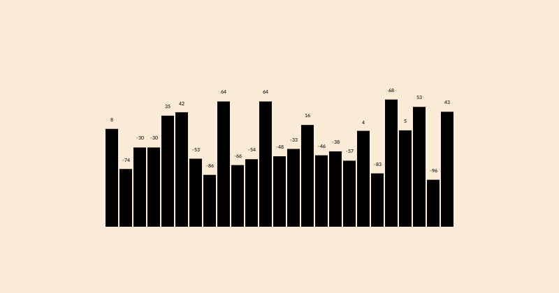
To change the way the bars and labels are drawn, define some functions and pass them as keyword arguments:
function mybarfunction(values, i, low, high, barwidth, scaledvalue)
    @layer begin
        extremes = extrema(values)
        sethue(Colors.HSB(rescale(values[i], extremes[1], extremes[2], 0, 360), 1.0, 0.5))
        csize = rescale(values[i], extremes[1], extremes[2], 5, 15)
        circle(high, csize, action = :fill)
        setline(1)
        sethue("blue")
        line(low, high, action = :stroke)
        sethue("white")
        text(string(values[i]), high, halign=:center, valign=:middle)
    end
end

function mylabelfunction(values, i, low, high, barwidth, scaledvalue)
    @layer begin
        translate(low)
        text(string(values[i]), O + (0, 10), halign=:center, valign=:middle)
    end
end

v = rand(1:100, 15)

bbox = BoundingBox() * 0.8
box(bbox, action = :clip)
p = barchart(v, boundingbox=bbox, barfunction=mybarfunction, labelfunction=mylabelfunction)

rule(p[1])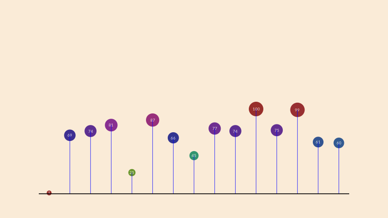
Box maps
The boxmap function divides a rectangular area into a sorted arrangement of smaller boxes or tiles based on the values of elements in an array.
This example uses the Fibonacci sequence to determine the area of the boxes. Notice that the values are sorted in reverse, and are scaled to fit in the available area.
You specify the top left corner of the graphic, the width, and the height.
fib = [1, 1, 2, 3, 5, 8, 13, 21, 34, 55, 89, 144]

# make a boxmap and store the tiles
tiles = boxmap(fib, BoundingBox()[1], 800, 450)

for (n, t) in enumerate(tiles)
    randomhue()
    bb = BoundingBox(t)
    sethue("black")
    box(bb - 5, action = :stroke)

    randomhue()
    box(bb - 8, action = :fill)

    # text labels
    sethue("white")

    # rescale text to fit better
    fontsize(boxwidth(bb) > boxheight(bb) ? boxheight(bb)/4 : boxwidth(bb)/4)
    text(string(sort(fib, rev=true)[n]),
        midpoint(bb[1], bb[2]),
        halign=:center,
            valign=:middle)
end